CCTBX.XFEL4MFX - Stable Compiling Github Issues documented by Fred and answers from chats with Aaron, Dan, David, and other cctbx.xfel developers. Adapted Pam’s notes of computational crystallography sessions and the 2025 Users’ Meeting tutorial document shared by Sandra. Louis has been critical for the parts on geometry from BayFAI and psana related code. As all software and the computing environments are updating all the time, please keep the timestamp of the document and the sections in mind. This stable version is meant for viewing only. If you want to make edits/comments, or you need bleeding edge updates, you can check out the “living” version of this handbook that contains the latest fixes and updates information, but expect the content to be messy there. Content highlighted in yellow means partially completed, work in progress.

Change log

• 02/03/26: Doris updated chapter “Intermediate: Prepare for real-time usage during beamtime (S3DF)” according to discussion with Fred and Pam.
• 01/29/26: Doris added chapters “Intermediate: Prepare for real-time usage during beamtime (S3DF)” and “Intermediate: Indexing result improvement” (mostly high-level guidance at this point) and a brief “Appendix: relevant programs and parameters”. Updated “Basic: CCTBX.XFEL Programs and Tasks” based on discussion with Pam and Vandana.
• 01/08/26: Doris added chapters “Intermediate: Photon energy calibration” (mostly complete, but no solutions for experiments that would throw errors), “Advanced: Event code handling”, and updated “Debugging tips”. Updated the “Within a Dataset, Defining Tasks” section to based on Selena’s progress. Added chapter “Intermediate: How to make a mask”.
• 12/07/25: Sandra improved the chapters “Remote access to GUI” and “Initial GUI configuration for an experiment”. Doris completed the chapter “Geometry Refinement”.
• 11/24/25: This is the very first release as an internal test.

• GUI source code: https://github.com/cctbx/cctbx_project/tree/master/xfel/merging
• Preprint: cctbx.xfel: a suite for processing serial crystallographic data
• Psana confluence page: https://confluence.slac.stanford.edu/spaces/LCLSIIData/pages/267391733/psana?macroName=view-file&desktop=true#psana-DetectorNames
• LUTE documentation: https://slac-lcls.github.io/lute/dev/
• BayFAI via LUTE documentation: https://slac-lcls.github.io/lute/dev/usage/tasks/bayfai/bayfai/

A note on copy/paste between your local computer and the remote session: shortcut keys can differ, so if paste fails, keep that in mind. For OnDemand, copy/paste between local (Mac) and the VNC session did not work at all.

S3DF: OnDemand (least lagging, but no copy/paste)

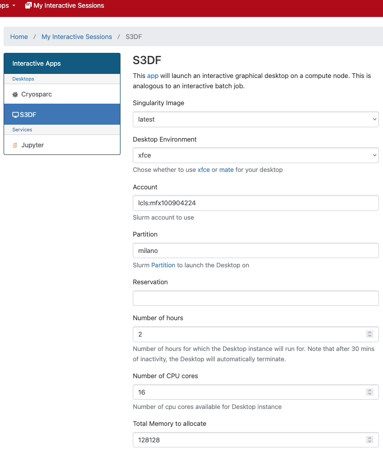
S3DF OnDemand: https://s3df.slac.stanford.edu/ondemand

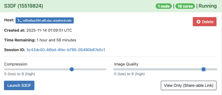
From there, open Interactive Apps in the top menu and choose S3DF. After it starts, you may want to lower image quality for responsiveness, then choose Launch S3DF.

NERSC: ThinLinc

Follow NERSC’s ThinLinc documentation: https://docs.nersc.gov/connect/thinlinc/ — it is fairly clear and straightforward (at least on Mac).

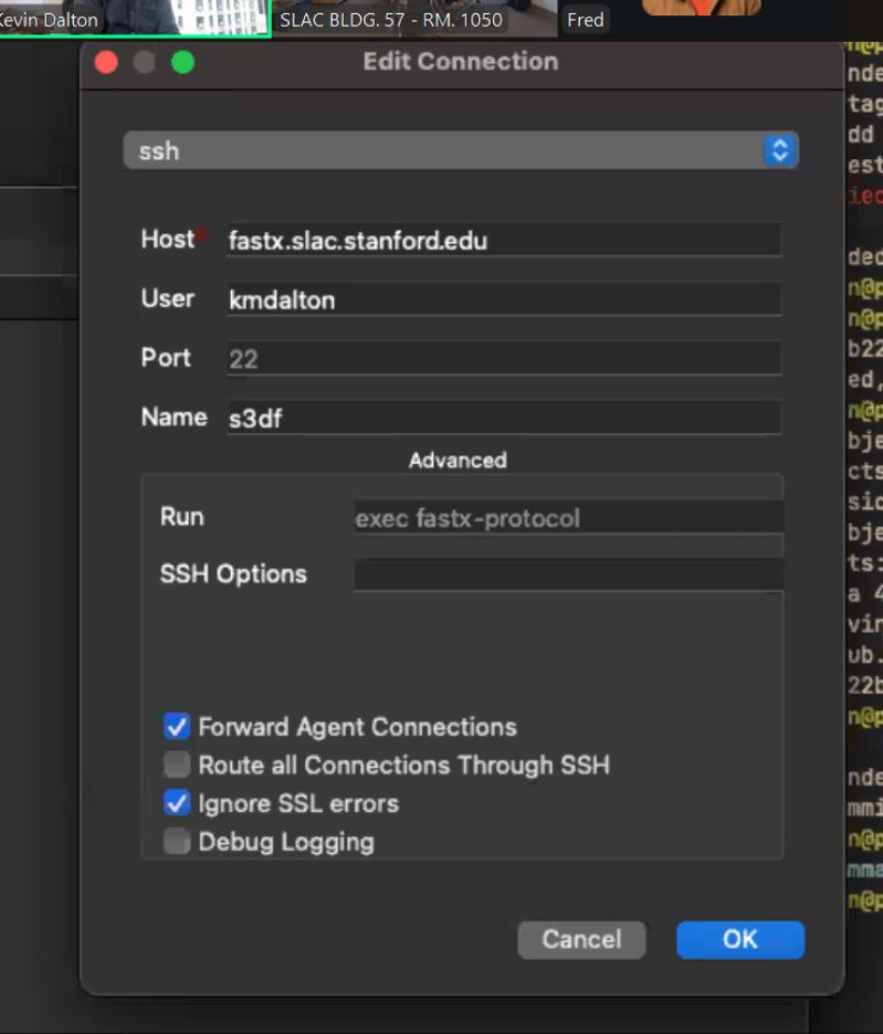
S3DF alternative 1: FastX v4 (StarNet)

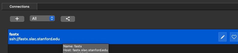
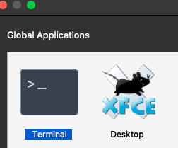
After saving the connection, double-click it. Enter your login credentials; you should see the usual S3DF prompt. Click the + icon at the upper left to start a new session. Choose Terminal rather than Desktop (this historically avoided a bad display issue with the GUI). In the terminal, ssh into psana.

S3DF alternative 2: NoMachine

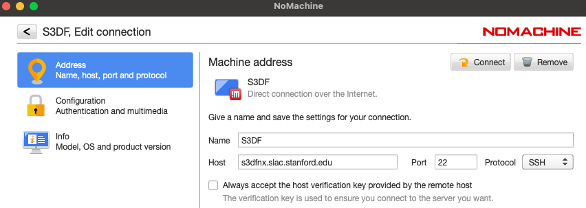
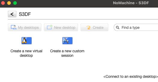
Click Add to create the connection. After saving, double-click the S3DF icon, then Create a new virtual desktop. Open a terminal in the desktop, then ssh into psana.

Other options (e.g. Xming) exist but can be very slow.

Login to the remote session via SSH

To enable graphics forwarding, use -Y when you ssh, for example:

ssh -Y <username>@s3dflogin.slac.stanford.edu

Depending on your SSH config, you may need an extra hop into psana:

ssh -Y psana

Source cctbx

On S3DF

• psana2: source /sdf/group/lcls/ds/tools/cctbx/psana2_setup.sh
• psana1: source /sdf/group/lcls/ds/tools/cctbx/psana1_setup.sh

Tips

• Avoid putting source in .bashrc (too aggressive for Python).
• Prefer a clean environment; even avoiding activating base Conda via .bashrc is good practice.
• setup.sh is a wrapper around conda_setpaths.sh from the cctbx build and sets required environment variables (they differ on S3DF vs NERSC).

If setup.sh is missing, create one. S3DF example:

export SIT_DATA=/sdf/group/lcls/ds/ana/data
export SIT_PSDM=/sdf/data/lcls/ds/
export SIT_ROOT=/sdf/data/lcls/ds
export SLURM_PRIORITY_RESERVATION=lcls.onshift
umask 002
source /sdf/group/lcls/ds/tools/cctbx/build/conda_setpaths.sh

On NERSC

source /global/common/software/cctbx/alcc-recipes/cctbx/activate.sh

Figures (from PDF)

0. Source the right cctbx environment

See Preparation → Source cctbx (SSH section above).

1. Configure experiment settings

The overall GUI configuration for an experiment lives in:

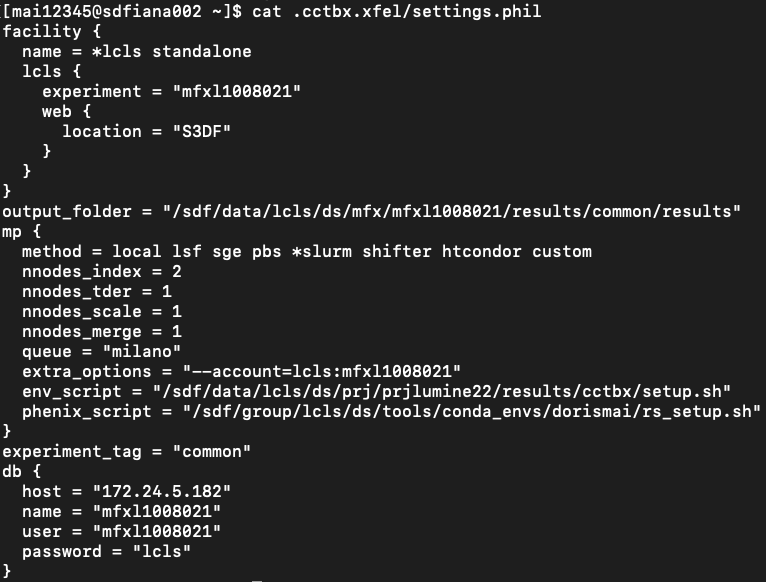
/sdf/home/<username>/.cctbx.xfel/settings.phil

That file pre-populates GUI fields, and edits in the GUI write back to settings.phil. If you have never run the cctbx.xfel GUI before, you may not have this folder or file yet.

If you switch experiments, the GUI can overwrite ~/.cctbx.xfel/settings.phil, so save a copy before running. You can copy an existing file as a template (create .cctbx.xfel if needed):

cp /sdf/home/<username>/.cctbx.xfel/settings.phil <experiment_file>

Example (Summers): /sdf/home/m/mai12345/.cctbx.xfel/mfx100904224.phil

The file content structure matches what the GUI shows (screenshots in Figures below).

You may start from scratch or from a partial settings.phil. If you set output_folder, those paths must already exist—the GUI will not create them and may crash or freeze.

2. Start GUI

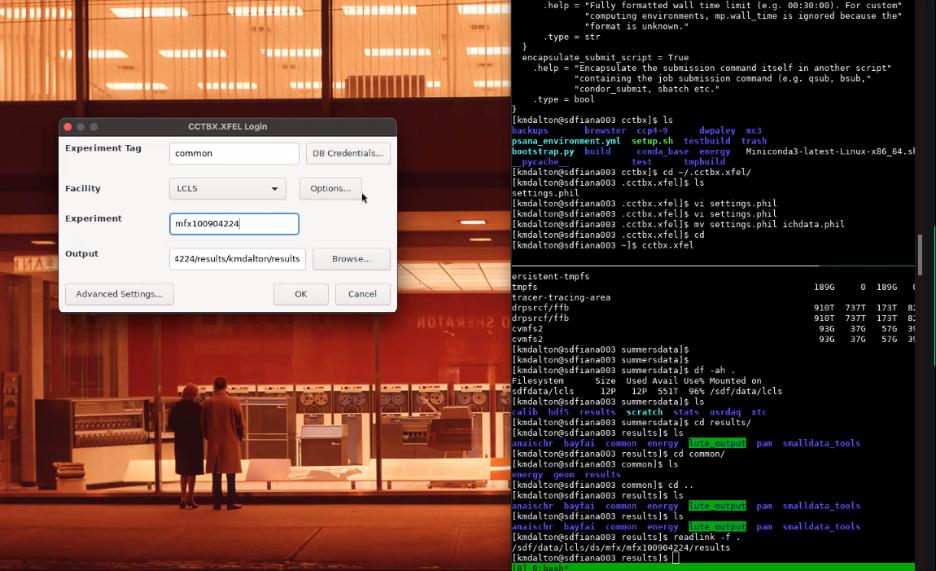
Run cctbx.xfel in a terminal (startup can take about a minute). With your PHIL loaded, you should see entries such as Experiment Tag (experiment_tag), Output (output_folder), Facility (facility.name), and Experiment (facility.lcls.experiment).

Fill any fields not already set from settings.phil.

Example output path shown in the GUI:

/sdf/data/lcls/ds/mfx/mfx100904224/results/kmdalton/results

Experiment tag and output folder

Conventionally the experiment tag and process folder (relative to the experiment folder) should match, but this is not always enforced. For example the tag may be common while the processing folder (relative path) is pam or kmdalton (as in the screenshots).

Unless you are the official processing person (in which case the output folder is usually common), create a folder for yourself (e.g. pam). The overall experiment folder is set by the facility layout; the GUI expects your processing folder as an absolute path.

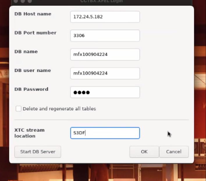
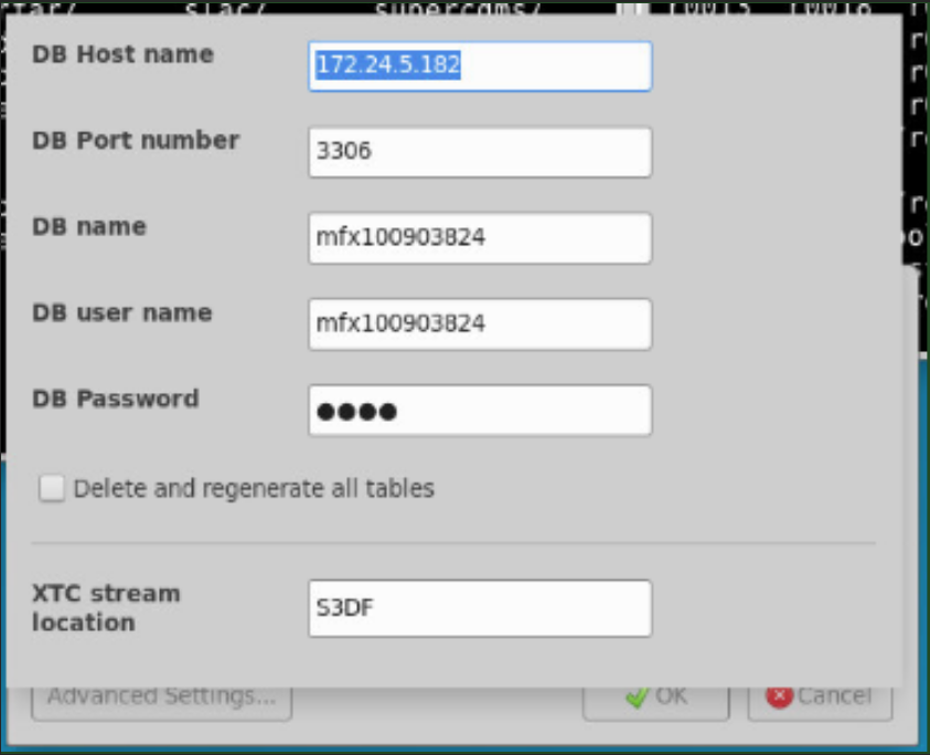
DB credentials

Match the db section in settings.phil. Name and user are usually the experiment. Password is often lcls.

If bottom buttons in the DB window disappear (e.g. via OnDemand), exit with Return or Escape.

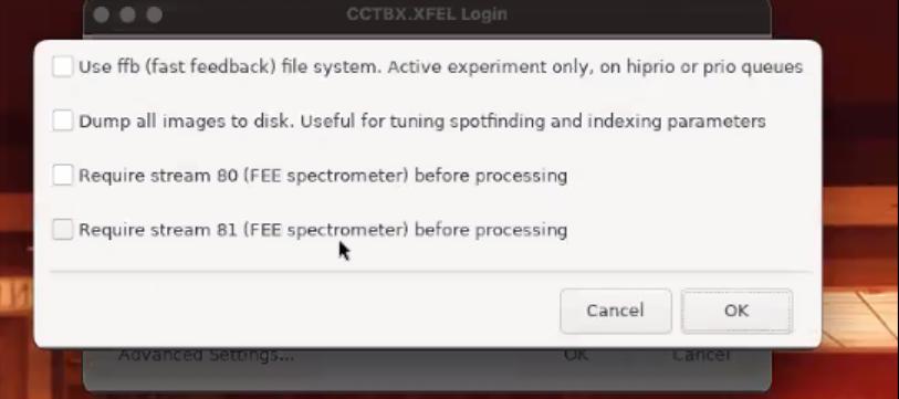
Options

Leave them unselected unless you know you need them.

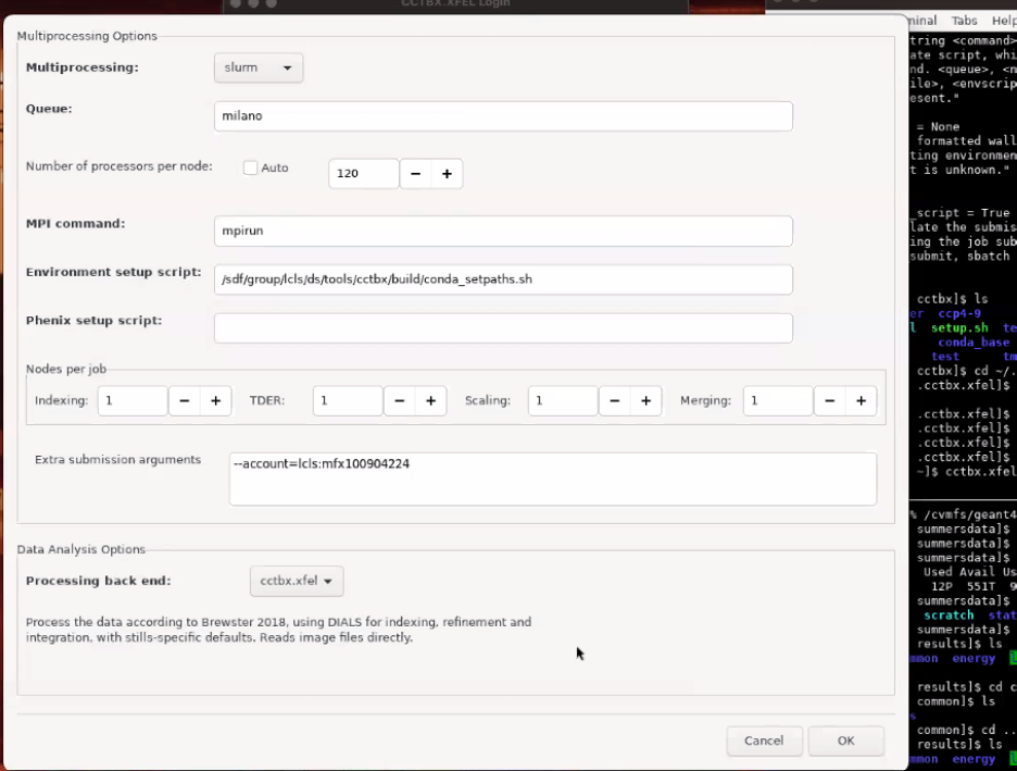
Advanced settings

Correspond to the mp section in settings.phil. The Environment setup script must match how you sourced cctbx in step 0.

Other fields are mostly Slurm-related, including Extra submission arguments (extra_options under mp as a string). Milano has 128 cores and WEKA uses 8—use at most ~120 processors per node. The Slurm account in extra arguments should match the experiment.

For real-time beamtime work you may add --reservation=lcls:onshift (higher priority, limited to 10 nodes—use sparingly).

3. Populating runs

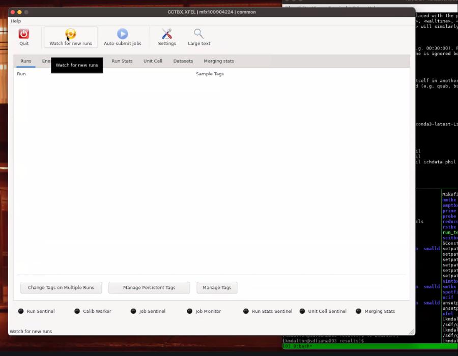
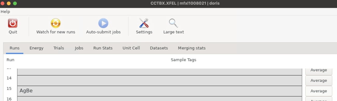
In the GUI, click Watch for new runs (hold until the button turns yellow). Buttons can lag.

Only one GUI instance should watch at a time—turn watch off when not needed. For reprocessing, a short watch is enough to load run metadata.

Runs should appear under the Run page.

4. Tagging runs

• Manage Tags — add tags.
• Change Tags on Multiple Runs — apply tags to many runs.
• Manage Persistent Tags — auto-tag incoming runs when the sample is stable (change when the sample changes).

If the GUI crashes during real-time processing, reconfigure persistent tagging after relaunch, or untagged runs can pile up.

Figures (from PDF)

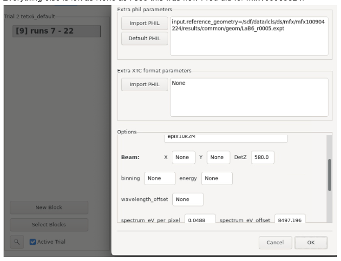
1. Defining Trial (i.e. Indexing parameters) Go to the “Trials” page of the GUI. This is a somewhat peculiar part of how the GUI is organized. When creating a trial, what you put in the big textbox is actually parameters for the Indexing task. However, all the other tasks are defined under Datasets (see step 2). The format/grammar of the content is the same as the phil file, which stands for Python Hierarchical Input Language (a kind of format used for cctbx and phenix programs): https://cci.lbl.gov/docs/cctbx/doc_low_phil/ Under the hood, the Indexing task is performed by calling the program dials.stills_process. If you don’t know what parameters are accepted by this program to put in the textbox, you can use dials.stills_process -ca 2 -e 10
   Similar command works for other cctbx/dials programs if you want to learn more about the parameters, and the flags specify the expert (verbose) level of the help messages. An example input looks like this: dispatch { hit_finder { minimum_number_of_reflections = 16 } } spotfinder { filter { min_spot_size = 2 max_spot_size = 100 } threshold { algorithm=dispersion dispersion { gain = 1 kernel_size = 1 1 global_threshold = 10 } } } indexing {

  stills.reflection_subsampling.enable=True

known_symmetry { space_group = P 1 21 1 unit_cell = 87.970 52.420 95.650 90 95.609 90 } refinement_protocol { d_min_start = 2 } multiple_lattice_search { max_lattices = 3 } }

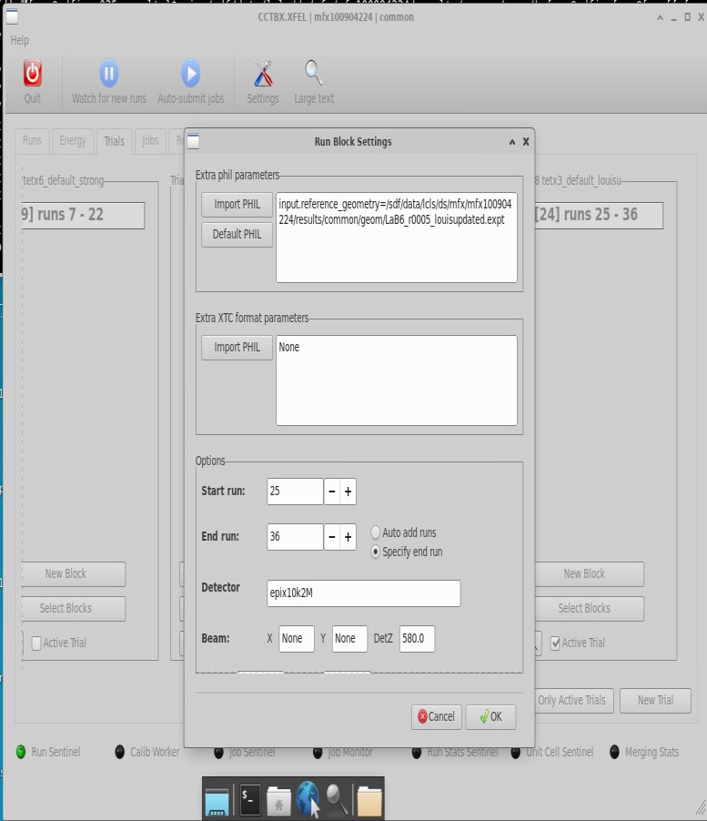
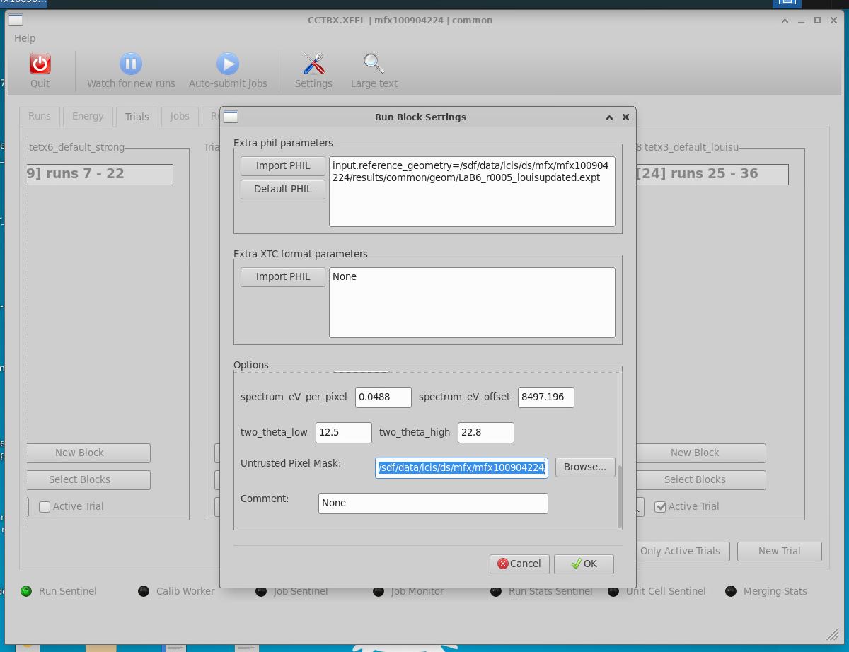
Remember to check space group and unit cell information here (and make new trials if necessary) if you have samples with distint values. During real-time processing, it could be helpful to add the line integrate = False within the dispatch block (above hit_finder) to speed up the indexing results. However, remember to either re-run (by making another trial) without this flag or perform ensemble refinement to make sure you can eventually do scaling and merging (See Section 3. Within a Dataset, Defining Task) Within a trial, define Run Group - You need to specify the start and end (inclusive) runs. For real-time processing, “Auto add run” can be helpful, but you need to remember terminate it by specifying the end run one sample is changed. - A path to .expt file that specifies the geometry (see step a below) at the top textbox.
- Under the second large text box “Extra XTC format parameters”, for psana2, you need to put the line “mode=psana2_idx”.
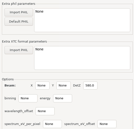
- Specify the detector name. If you don’t know exactly the format, the detnames program from psana is helpful (see the Debug chapter). - Specify binning, if any - Put in the spectrum_eV_per_pixel and spectrum_ev_offset values if you have that (see the Photon energy calibration chapter). You can either manually input them, or if you have saved the .phil from photon energy calibration, or use the “Import PHIL” button to populate the values from the file for you. - Load the pixel mask (see step b). If you don’t know how to make mask, see the corresponding chapter.

a. For each run group specify the geometry file For the example experiment we look at, the detector calibration was performed using LaB6. The experiment file can be found here:

/sdf/data/lcls/ds/mfx/mfx100904224/results/common/geom/LaB6_r0005_louisupdate d.expt This will be input.reference_geometry in the run block settings The .expt file will overwrite the values in the text boxes below for “Beam: X Y DetZ” b. For each run group load pixel mask For the summers experiment a mask can be found here:

/sdf/data/lcls/ds/mfx/mfx100904224/results/common/pixels.mask 

This can be used in the following

c. Extra XTC format parameters Other than specifying mode for psana2, if there are any issues of the XTC files, this textbox is likely where you need to modify, such as specifying spectrum address, putting a wavelength fallback value when eBeam is missing etc. Content in this textbox will be part of the data.loc file that enables retrieving and viewing the images.

d. Check this trial as the active trial, and uncheck other if you previously have other processing. 2. Defining Datasets
Go to the “Datasets” page of the GUI. Refer to “Tagging runs” in the previous chapter step 3 “Populating runs” if you have no clue about tags.
Depending on how you tag the runs, select if you want the intersection or the union of the tags to process a dataset. Intersection makes sense if say you have one tag of mixing time and another tag for temperature. Union makes sense if you want to combine runs that are similar (e.g. tagged by different delivery speed but otherwise the same sample). Not all runs defined by the tags you choose will be processed – only runs within the run groups of the trial will be used to look at tags. For example, run 1-40 are all tagged as apo, but your run group under the trial is defined as run 20-40, then the apo dataset will only process run 20-40. See below on task definition to see where trial comes in.
The name of the dataset will become the name of the folder for the Merging task.
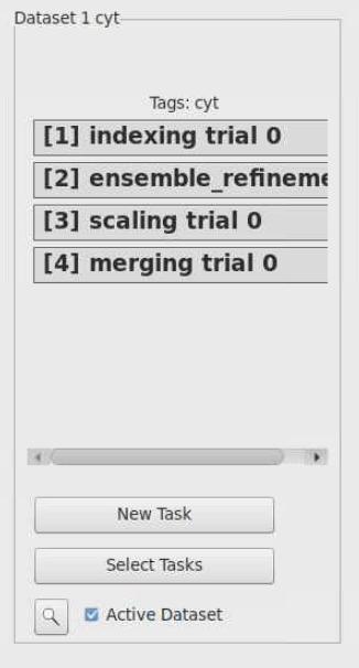
Do NOT contain space or weird characters in the dataset name, as merging can fail. Use a single word (linked by underscore is fine). Check this dataset as the active dataset, and uncheck other if you previously have other processing. 3. Within a Dataset, Defining Tasks Each task has to be associated with a specific trial. Under a dataset, click “New Task” to add a task and specify the trial and the parameters (PHIL format) for that task. ”Typically, you would have the following 4 tasks to run for a dataset:

The tasks you define are chained in the listed order, such that for a particular run, a local task (e.g. scaling, see explanation below) won’t run until the previous local task finishes. Ensemble refinement is an optional task, so you could just chain a scaling task right after the indexing task.
You might notice that in practice, after you define the trial and run groups, with the “Auto submit jobs” button on, indexing jobs can be automatically submitted for those runs, even if you haven’t defined the Indexing task. That said, you must define the Indexing task explicitly in the Dataset and chain the other tasks (such as shown in the screenshot above) in order to run the other tasks. For example, you cannot leave only Scaling and Merging tasks there, even if you have already got Indexing and Ensemble refinement results from previous processing. Technically you can chain Indexing task directly to Scaling task. However, make sure you did NOT set integrate=False for Indexing (which, remember, is set when you define the trial and cannot be edited).

Task Output Folder Structures Local task Indexing, ensemble refinement, and scaling are all considered local task, meaning the task is performed at the level of each run, and the outputs are organized under each run. A typical run folder structure (relative to experiment folder path) is this: r0023/002_rg015 Which means the ouput is for run 23 processed from indexing parameters in trial 2 and other information (e.g. geometry and pixel mask and energy calibration) associated with run group 15. The non-indexing local task has its own output folder named by the task id its assigned by the GUI, e.g. r0023/002_rg015/task009 Global task
Merging, however, is a global task as it is performed across runs. The output folder is named by the dataset name, and lives in the experiment folder where each run folder lives. This task will be run for many versions, as the previous local task (scaling) finishes for more and more runs. See the “Outputs” subsection under the “Merging” section below for more details.

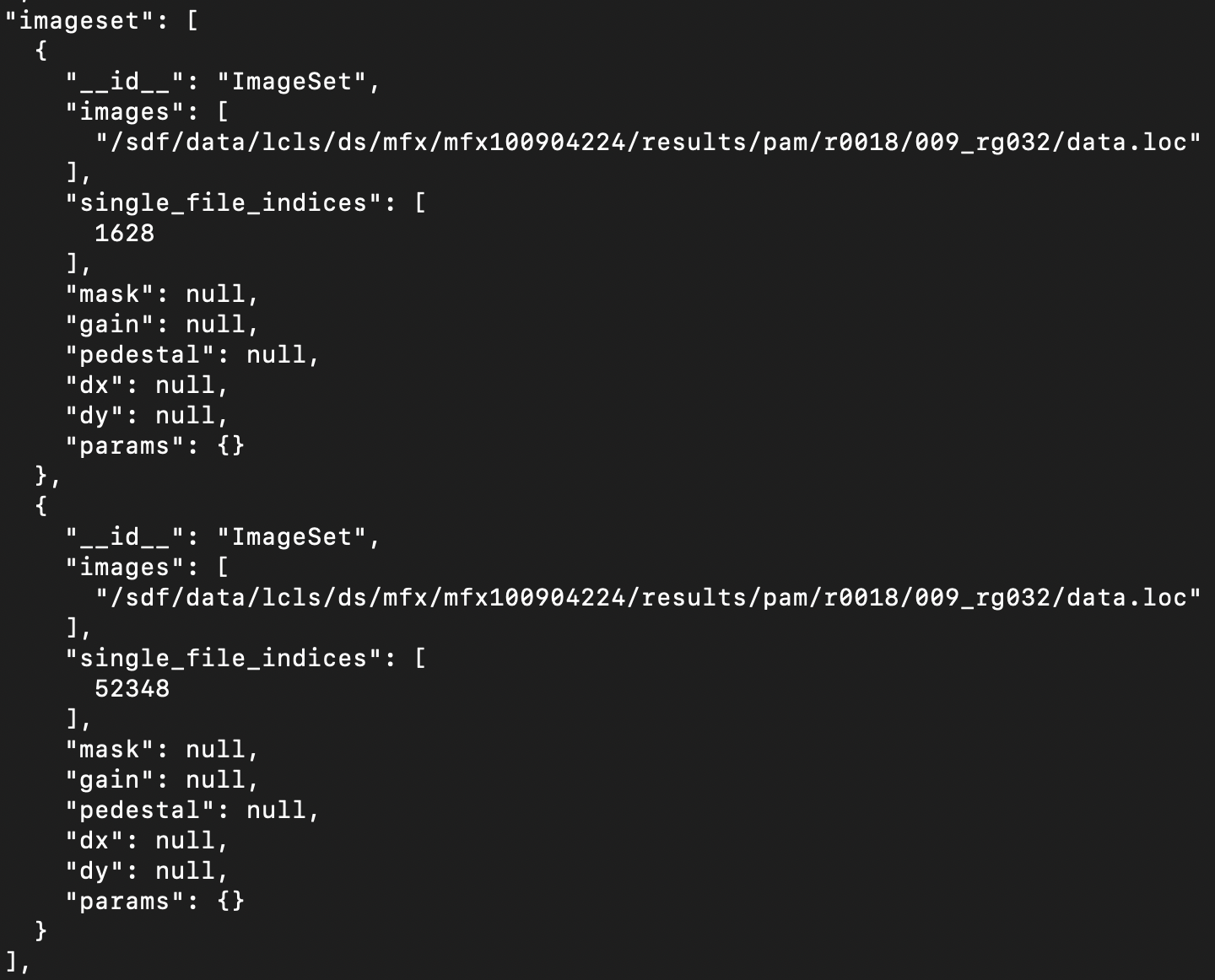
Indexing See step 1 for trial definition. You don’t need to put any parameters here. Outputs: Within the run folder, you would have a data.loc file, out folder, stdout folder, a params_1.phil file, and slurm job submission script submit.sh and its wrapper submit_submit.sh. The out folder contains the .expt and .refl outputs. One idx-{number}_refined.expt file does NOT necessarily mean 1 image – it could contain multiple images:

The “single_file_indices” tells you the actual index of the image. In other words, if you are viewing all images (including non-hit) of the entire run using dials.image_viewer data.loc load_models=False, you can jump to view the same image using this index (+1, apparently 0-indexed). To just view some example of indexed images, you could do dials.image_viewer idx- {whatevernumber}_*.{expt,refl} load_models=False Errors of the job would end up in the stdout folder although it is very hard to debug (especially mpi related) errors based on messages there. I usually only look at the err.out file there. The parameters you put under trial definition would end up in params_1.phil. “Extra XTC format parameters” would end up in data.loc, which used by the GUI to talk to psana and get images data. See the chapter “Intermediate: Indexing result improvement” for more details on checking the indexing statistics and strategies for improvement.

Ensemble refinement Refines the geometry, unit cell, etc. and performs integration.
Example inputs combine_experiments.clustering.use=False reintegration.integration.debug.output = True reintegration.integration.debug.separate_files = False reintegration.integration.mp.nproc = 32

reintegration.integration.summation.detector_gain = 0.46

You may want to change the detector _gain in the last line depending on the type of detector (e.g. 1 used for Epix10ka2M).

Outputs: Within the task output folder (e.g. r0023/002_rg015/task009), it has another folder like combine_experiments_t002, where t002 means trial 2. Within this folder, you two folders final_extracted and intermediates. The integration results (.expt and .refl files) as well as log files are in the intermediates. Scaling Scaling and Merging both use cctbx.xfel.merge program, and it’s the dispatcher list that decides what processing is actually performed. An example phil parameters for scaling is attached below. As you can see, “scaling” is there, but it really is just one of many steps needed to perform for the Scaling task. Example inputs dispatch.step_list=input balance model_scaling modify filter errors_premerge scale postrefine statistics_unitcell statistics_beam model_statistics statistics_resolution input.parallel_file_load.method=uniform filter.outlier.min_corr=-1

filter.algorithm=unit_cell filter.unit_cell.value.relative_length_tolerance=0.01 
select.algorithm=significance_filter select.significance_filter.sigma=0.1 

select.significance_filter.min_ct=200

select.significance_filter.max_ct=300

scaling.model=/sdf/data/lcls/ds/mfx/mfxl1008021/results/common/models/

L10080_no_mix_rsich_refine_6.pdb scaling.resolution_scalar=0.96

merging.d_min=1.2

merging.merge_anomalous=True postrefinement.enable=True statistics.n_bins=20 

output.save_experiments_and_reflections=True Outputs: The task output folder is structured very similar to the indexing output folder (one level up of this task output folder), except that there is not data.loc file here. Merging Example inputs dispatch.step_list=input model_scaling statistics_unitcell statistics_beam model_statistics statistics_resolution group errors_merge statistics_intensity merge statistics_intensity_cxi publish input.parallel_file_load.method=uniform scaling.model=/sdf/data/lcls/ds/mfx/mfxl1008021/results/common/models/ rsich_high_dmso_150ms_mixing.pdb scaling.resolution_scalar=0.96

statistics.n_bins=20 
merging.d_min=1.28 
merging.merge_anomalous=True merging.error.model=mm24 

To upload merged .mtz files into google drive, refer to this instruction to set up (https://github.com/cctbx/cctbx_project/tree/master/xfel/merging/application/publish), and add two more lines in the inputs: publish.drive.credential_file= publish.drive.shared_folder_id=

Additional notes If you don’t specify the google drive related parameters to publish mtz files but you have publish in your dispatch.step_list, the merging job will finish with a status “EXIT” which normally indicates something went wrong wit the job, but here it could be fine. You can check the err.log the output folder to confirm it is this type of error that led to EXIT, and you should still have all the other proper output files. If you are looking at some old processing data, you might see phil parameters like merging.error.model=ev11 merging.error.ev11.algorithm= This was prototype (deprecated) code and is transitioned to mm24 now.

Outputs: Within the output folder (named after the dataset, lives under the experimental folder), there are many versions as more runs coming in. For final result, you want to look at the folder with the largest version number. Within this folder, the key files are: - {dataset_name}_v{version_number}_main.log: contains merging stats - {dataset_name}_v{version_number}_all.mtz: overall merged output - {dataset_name}_merging{task_id}_v{version_number}_params.phil: your input parameters - {dataset_name}_merging{task_id}_v{version_number}_submit.sh There are also a lot of other logging files, including log.out and err.out, and wrapper submit script for slurm.
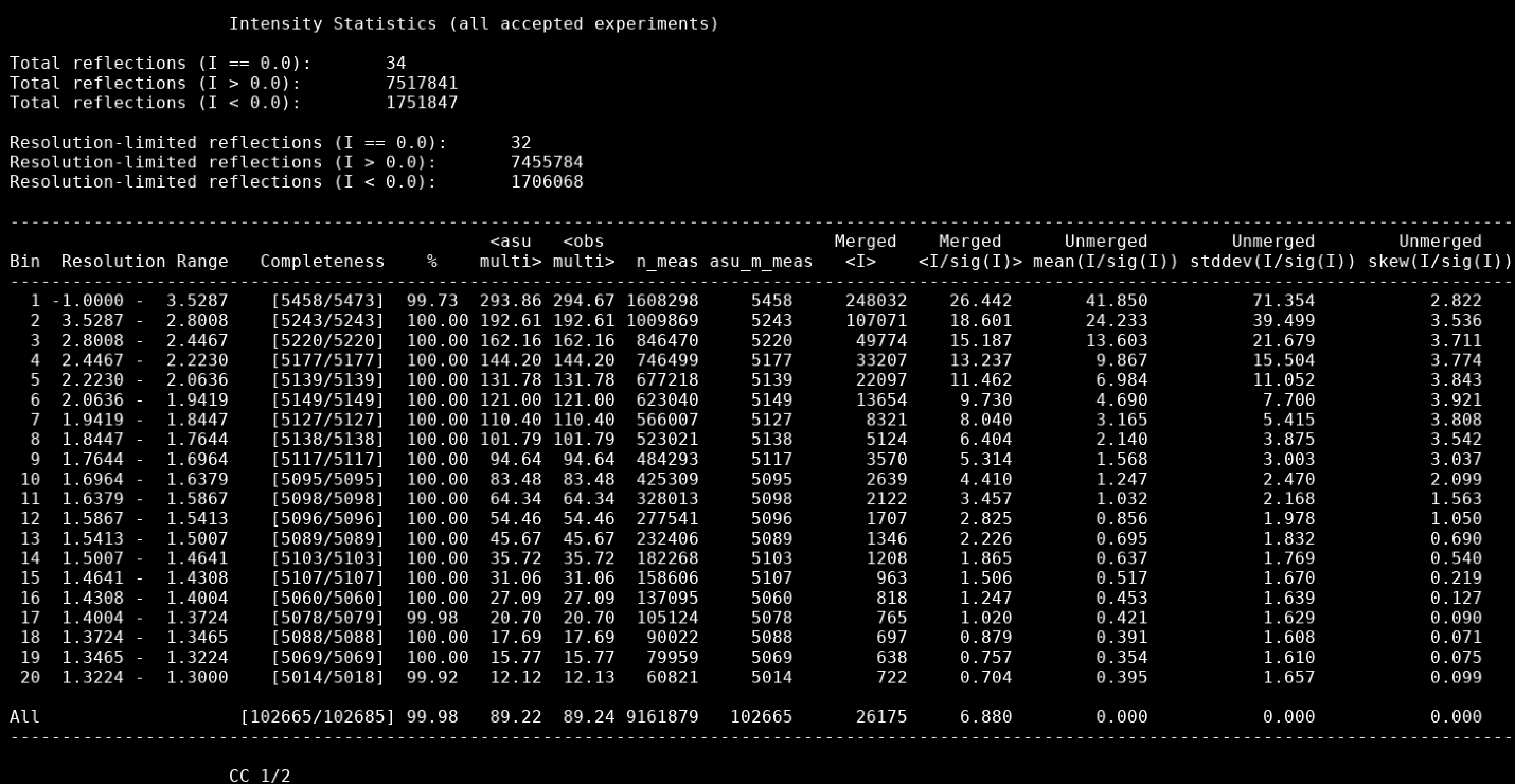
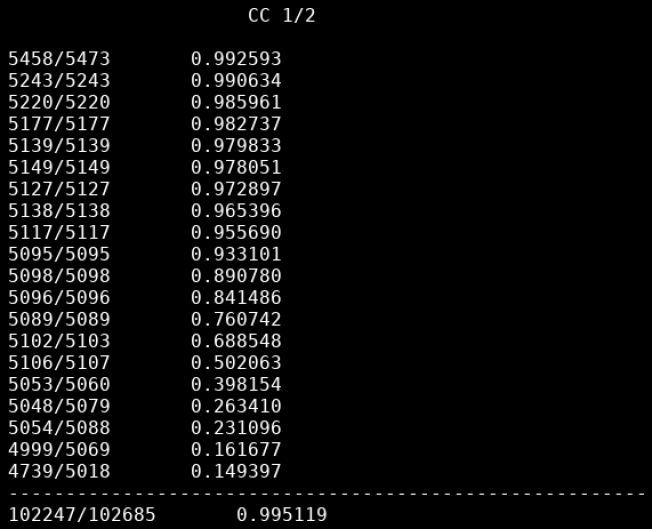
For quick triage I would mainly focus on the tables shown below in the …main.log file. The tables for all (rather than for odd/even) are closer to the end of the file. I would look at obs_multi > 10, CC1/2 > 0.3, and other metrics to decide resolution and if any pathology.

Quick Workflow Checklist 1. Connect via FastX 2. ssh -Y into S3DF 3. Source env:

 source /sdf/group/lcls/ds/tools/cctbx/setup.sh 

4. Copy .phil settings
5. Start GUI → enter experiment info
6. Configure DB credentials
7. Set options + advanced settings
8. Start processing (watch new runs or manual selection)

9. Geometry calibration and energy calibration, in either order

10. Make/load Pixel Mask

11. Define trial, run groups if not already
12. Define dataset
13. Start an indexing task (or more)

Figures (from PDF)

Before the beamtime

General

• Check that the experiment folder has been set up on S3DF and is visible on eLog.
• Collect dark runs (test takepeds/makepeds).
• Collect calibrant data and run BayFAI (during commissioning).

Note on BayFAI / geometry (2026/02)

See the LUTE documentation for setting up and running BayFAI to estimate geometry: https://slac-lcls.github.io/lute/dev/usage/tasks/bayfai/bayfai/

As of 2026/02, this means following the linked instructions in the experiment folder. After setup, the BayFAI workflow should auto-populate on eLog → Workflow → Definitions; adjust as needed (e.g. set Trigger to MANUAL rather than end of run, tune Slurm arguments such as --ntasks).

Database

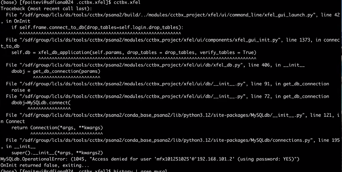
• Users must request MariaDB on their form to use the cctbx.xfel GUI. If that is missing, email pcds-datamgt-I to set it up.
• If the GUI shows a database error on launch, the DB is not ready yet.

Verify with:

mysql -h 172.24.5.182 -u <experiment> <experiment> -p

See Debugging tips for more mysql commands.

GUI readiness

Run test jobs (e.g. energy calibration) before beamtime:

• Can you launch the GUI (remote access + sourced cctbx)?
• Can the GUI reach MariaDB and show runs under Watch for new runs?
• Can you submit simple jobs (e.g. average a run and view the image)?

Analysis info to have ready

• Unit cell and space group; reference PDB if available.
• A PHIL template for indexing/trial definition (from users or a recent beamtime).
• Optional: reference geometry .expt (if not using BayFAI).
• Optional: reference mask from a recent beamtime.

During the beamtime

The main question is whether enough data exist to move on. Ideally you reach merged results and inspect stats; in practice, indexed image count is a quick gauge.

Make initial files for indexing

• No geometry yet → average a run and create one.
• No mask yet → average a run and build one.

Initial geometry/PHIL are rarely perfect; expect iterations on energy calibration, geometry refinement, mask updates, and spot-finding PHIL—similar to offline reprocessing.

Hit / indexing progress

Watch Run Stats and Unit Cell for indexing rate and counts. Tips:

• Use a persistent tag for incoming runs when the sample is stable (change it when the sample changes).
• Set integrate=False on the trial for indexing-only; remove it or run ensemble refinement before scaling/merging.

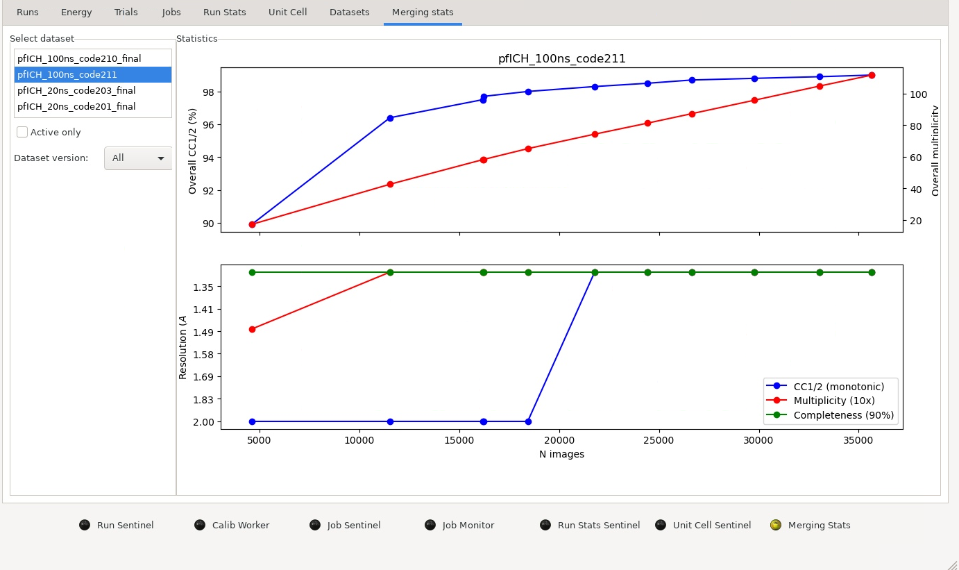
Merging progress

Use the Merging stats tab. Active only refers to the dataset (optional). Leave Dataset version as All to see stats evolve across versions.

Do not pick a single dataset version—plotting can fail (Merging Stats sentinel turns red). Switch tabs and return, or relaunch the GUI to recover. Plotting can be slow; watch the sentinel: if it stays idle and does not go yellow (working) or goes red, it may be stuck.

You want metrics to rise and then plateau when data are sufficient. Do not mix different samples in one dataset or trajectories become misleading. This tab is for “do we need more data?”; for full merging statistics, use the ...main.log file in the merging output folder.

Figures (from PDF)

cctbx/dials understands the geometry through psana. If BayFAI was used to estimate detector distance, it will push the result to a database such that psana2 Datasource can retrieve information from it, and this is how cctbx will understand the initial geometry. For psana1, this depends on the file written by BayFAI to the calib folder of the experiment: /sdf/data/lcls/ds/mfx/{experimentname}/calib. This file is still written for psana2 BayFAI but is just for logging purpose as the database is the way to communicate with cctbx now. Without BayFAI, psana use the default metrology data. Obtaining an initial geometry .expt file Average a run If cctbx can retrieve images and geometry from psana properly, you would first click “Average” for the calibrant run to make powder:

Under the hood, averaging a run uses geometry from psana, which could come from BayFAI or default metrology. The status of the average job is not checked in GUI under jobs, but actually in the terminal like your regular slurm job submission.
Once averaging is done, go to the output folder, should be output path like:

/sdf/data/lcls/ds/mfx/{experiment_name}/results/{experiment_tag}/averages/000 

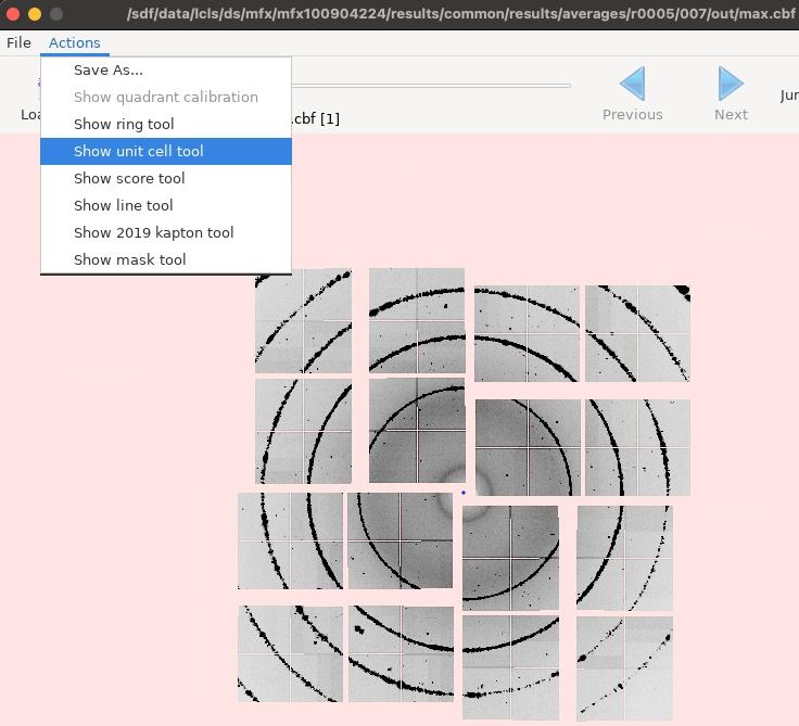
If you see more folders like 000, 001, … these are different versions of averaging done for this run. Within a version folder, you should have data.loc, submit.sh, submit_submit.sh (wrapper submit script), and the out and stdout folders. In the out folder, you should have max.cbf, std.cbf, and avg.cbf. I find it easier to work with max.cbf for geometry stuff, and std.cbf for masking.

Generate an initial .expt file In the terminal at the out folder:

dials.import max.cbf wavelength=1.4443 

By default it generates a file named imported.expt.

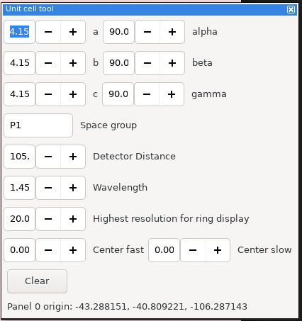
Visualize in dials.image_viewer the geometry fit Launch image: dials.image_viewer imported.expt If the calibrant is LaB6 rather than Agbe, add the following to the command above: unit_cell=4.15,4.15,4.15,90,90,90 After you have the image viewer pop up, click “Actions” –> “Show unit cell tool”, which would pop up another window.

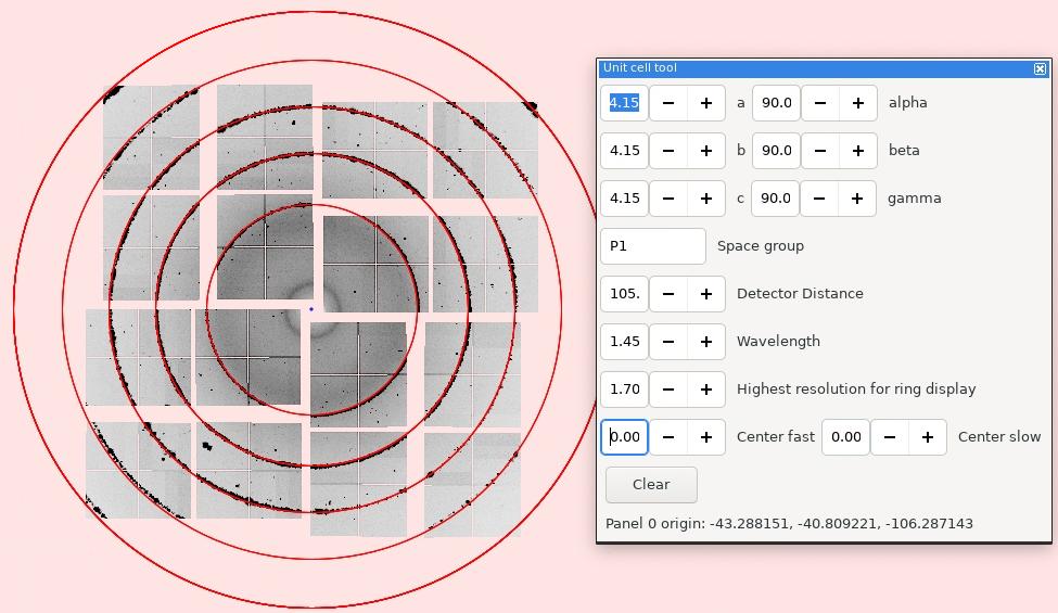
1. Lower the “Highest resolution for ring display” and hit enter to show the rings. In this case, 1.7 is a good value to display rings to the edge of the image.

2. If the red rings are a bit off with respect to the actual powder signals, you can explore some manual fitting here through “Detector Distance”, “Center fast” (x-axis, positive points to right), “Center slow” (y-axis, positive points down).
   Notes and tips: - The “Detector Distance” is auto-populated through the .expt file from psana geometry, but in practice we have seen some discrepancy between the values. Generally speaking, as long as the fit looks good, you can proceed and give indexing a try. See “Understand the detector distance number” section below for more details. - If you manually refine the distance or the X/Y position in the “Unit cell tool” window, it won’t be saved to the .expt file. You would need to edit the values in the corresponding section in the .expt file. See “Understand the detector distance number” and “Modify beam X/Y (Center fast/slow)” sections below for more details. - If you mis-enter something of the wrong format, the image viewer could just crash/freeze, you would have to start over. Understand the detector distance number As of 2025/11, there is some weird discrepancy between the value in the .expt file and the value populated in dials.image_viewer. We don’t fully understand why, but at least for mfx100904224 run 5 it seems okay enough to have some indexing results and refine geometry further.

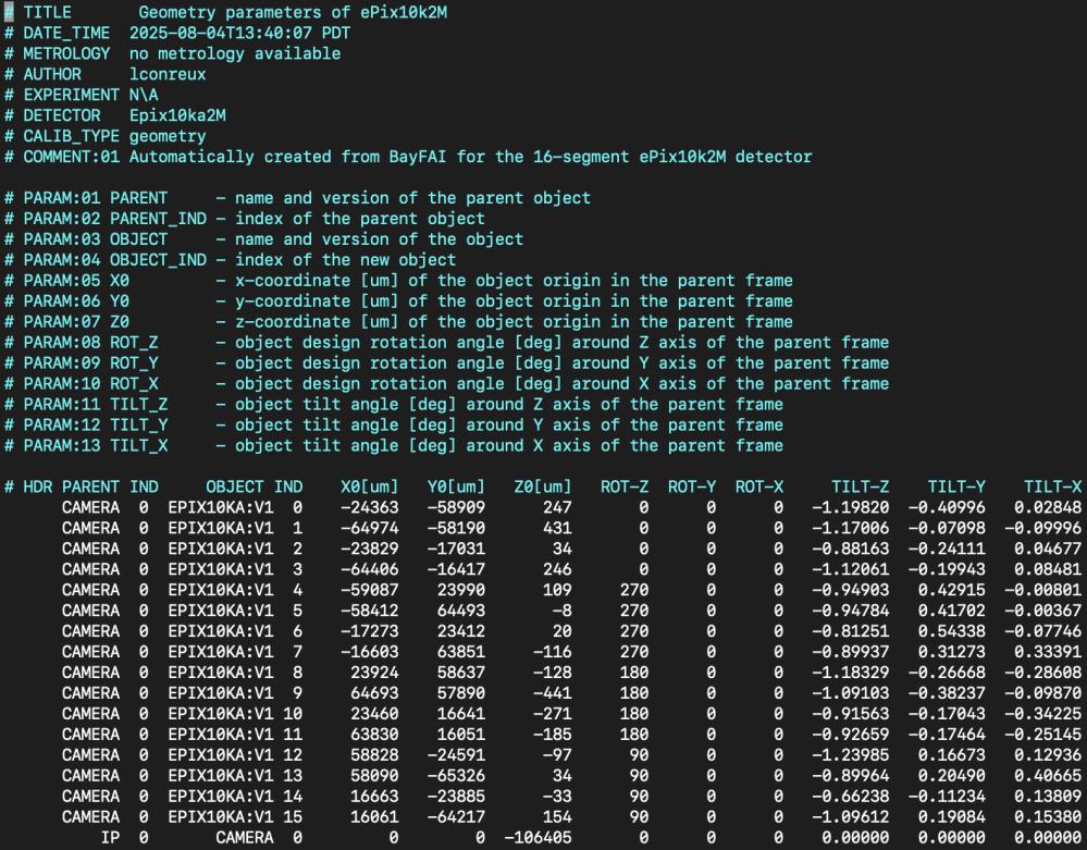
Psana convention is to output detector distance as a negative number, and this is the convention followed by BayFAI. dials.import direcly puts this negative number into the .expt file. You can check this distance in the {run_number}-end.data, which is written by BayFAI to the calib/{detectorname}/{somemoredetetctorname}/geometry/ folder. An example file is: /sdf/data/lcls/ds/mfx/mfx100904224/calib/Epix10ka2M::CalibV1/MfxEndsta tion.0:Epix10ka2M.0/geometry/5-end.data Look at the last line that begins with “IP”, in this case the distance would be –106.405 (converted to mm).

And in the imported.expt file, the corresponding line about detector distance is:

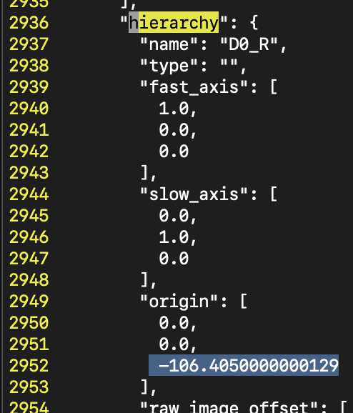
It would be the last number under “origin” under the first entry named “D0” or something similar immediately after “hierarchy”. Weird things we have observed as of 2025/11: - The plus/minus sign matters. In dials.image_viewer, a positive number is always enforced. However, it appears that the handedness of coordinate system is preserved. If bayFAI says –106.4, but you manually remove the minus sign in .expt file, the image would flip upside down in the dials.image_viewer. - There is some strange offset between .expt value and the value populated in the image viewer. For example, with –106.4 for mfx100904224 run 5, this is populated as 105.6 in the image viewer, but with 106.4 it is populated as 106.8. Modify beam X/Y (Center fast/slow) If you need to adjust the Center fast/slow entries in the “Unit cell tool” window of the image viewer, you need to save this result somehow by manually editing the .expt file. Suppose you need to adjust 50.0 and 40.0 for Center fast/slow.
Next you need to find the “pixel_size” in the .expt file. Do not look at the values near where you find the detector distance, as values would be 0 – instead, look for pixel_size near the top of the .expt file. In this case, it is [0.1, 0.1]. Then, multiply the values: this means that you would put down 5.0 and 4.0 instead of 50.0 and 40.0.
The plus/minus sign, as mentioned above in the detector distance section, can be tricky. In the image viewer, you would find positive as going right and down, but because of the discrepancy between psana and cctbx coordinate system (as of 2025/11), positive in the .expt file means going left and down.

Putting together, this means that you would modify the “origin” in the screenshotted part of the .expt file from [0.0, 0.0, -106.405…] to [-5, 4, -106.405,…].

Refine the geometry with DIALS Once you can successfully index some images, you can refine the geometry further using the indexed reflections. If needed, you can also refine the geometry again after running the ensemble refinement task (just update the file paths to point to ensemble refinement outputs rather than indexing outputs).

Use the first run in the run group we care about (e.g. run 21 for run group 58 trial 9 in this case). 0. Book-keeping: go to the geom folder – make one right under the experiment tag folder (e.g. common) if you haven’t, e.g. /sdf/data/lcls/ds/mfx/mfx100904224/results/common/geom. Then, make a refine folder for the run group (e.g. refine_rg058) and go into this folder. 1. combine the indexing output files:

dials.combine_experiments /path/to/expt /path/to/refl [optional arguments] 

For example, in the geom folder:

dials.combine_experiments ../../results/r0021/009_rg058/out/*refined*.

expt ../../results/r0021/009_rg058/out/indexed.refl reference_from_experiment.detector=0 output.n_subset=1000 output.n_subset_method=n_refl 2. Filter reflections: cctbx.xfel.filter_experiments_by_rmsd combined.* 3. Make a 0-level refinement phil file: or copy a previous one over: cp /sdf/data/lcls/ds/mfx/mfx100903824/results/common/geom/refine_rg011/re fine_level0.phil ./ Example 0-level refinement phil file looks like this: output.experiments=refined_level0.expt output.reflections=refined_level0.refl refinement {

parameterisation {
auto_reduction {
min_nref_per_parameter = 3
action = fail fix remove
} beam {
fix = all in_spindle_plane out_spindle_plane wavelength
}
}
refinery {
engine = SimpleLBFGS LBFGScurvs GaussNewton LevMar SparseLevMar
}
reflections {
outlier { algorithm = null auto mcd tukey sauter_poon separate_experiments = False separate_panels = True
}
}
}

You might want to explore the outlier algorithms. 4. Perform 0-level refinement on the filtered reflections:

dials.refine filtered.* refine_level0.phil 

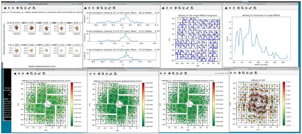
5. Visualize the results and log the terminal output: cctbx.xfel.detector_residuals refined_level0.* hierarchy=0 tag=refined Example figures output:

Generally, we care more about the bottom row of figures, with the following rule of thumb: - The greener plots the better - The lower left three figures should have spots cover the detector well to the edge - The “refined ΔΨ” figure should have spot concentrated into a small circular region in each panel center

Example terminal output: RMSD (microns) 150.5531824354221 Histogram mode (microns): 132.32253458087138 Overall mean (microns): 133.50295828414986 Overall median (microns): 127.85311020060347 Rayleigh Mean (microns) 165.84170327562524 Rayleigh RMSD (microns) 187.13232301185118 Overall radial RMSD (microns) 125.05808894584378 Overall transverse RMSD (microns) 83.82401144692689

6. Perform 1-level refinement and check the visual results and RMSD improve.
   Example 1-level refinement phil file: output.experiments=refined_level1.expt output.reflections=refined_level1.refl refinement { parameterisation {
   auto_reduction {
   min_nref_per_parameter = 3
   action = fail fix remove
   } beam {
   fix = all in_spindle_plane out_spindle_plane wavelength
   }
   detector { fix_list = Group1Tau1 hierarchy_level = 1 } }
   refinery {
   engine = SimpleLBFGS LBFGScurvs GaussNewton LevMar SparseLevMar
   }
   reflections {
   outlier { algorithm = null auto mcd tukey sauter_poon separate_experiments = False separate_panels = True

}
}
}

The command to visualize at level 1 is: cctbx.xfel.detector_residuals refined_level1.* hierarchy=1 tag=refined_h1

Figures (from PDF)

This chapter assumes you have basic familiarity with dials.image_viewer and you know how to average a run. Refer to the previous chapter “Geometry Refinement” if you are not familiar with them. Visualize a mask Given a pre-made mask (pixels.mask), you can visualize it on an image (std.cbf):

dials.image_viewer std.cbf load_models=False mask=pixels.mask show_mask=True 

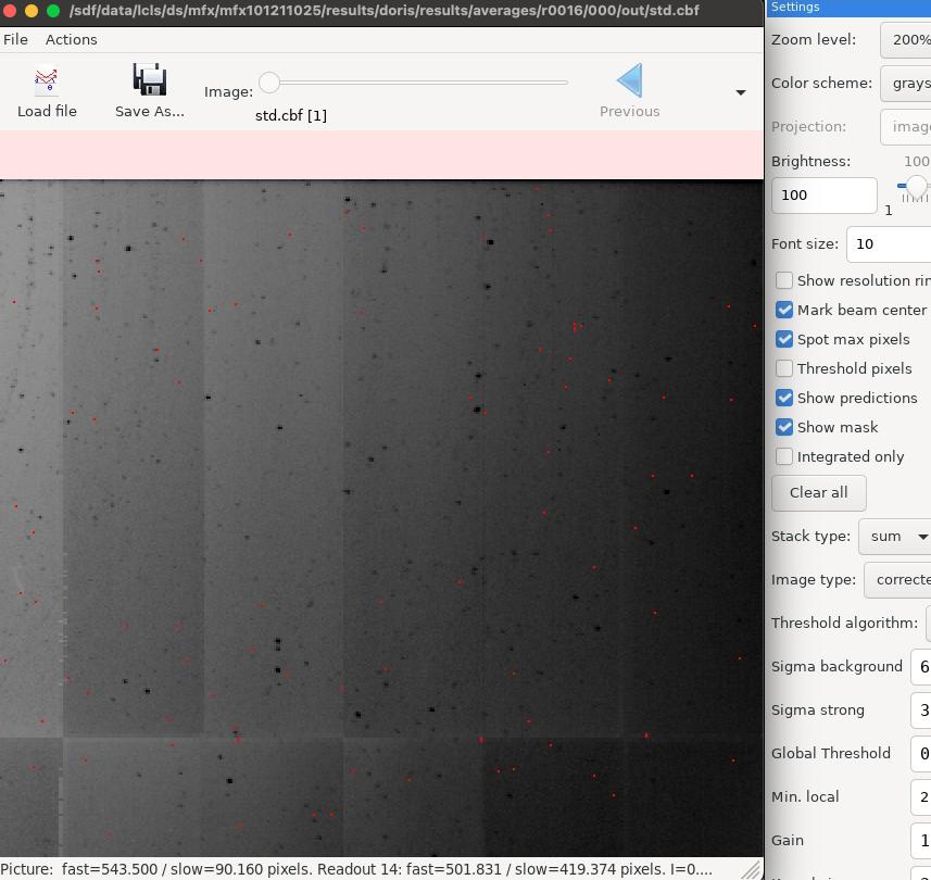
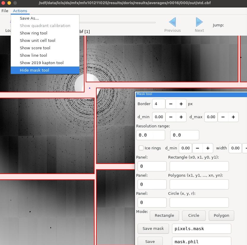
If you didn’t specify show_mask=True, remember to check the box for “Show mask” in the “settings” panel that pops up, and the masked pixels will be displayed as red. Make a mask Steps 0-4 describe how to make masks. After averaging a run, go to the output folder in the terminal. In the following example, the folder is

/sdf/data/lcls/ds/mfx/mfx101211025/results/doris/results/averages/r001

6/000/out, a case that requires extensive masking. 0. Dead pixels If pixels have 0 standard deviation, they are probably dead pixels. To make a mask of them, use the following script from Fred: (base) [mai12345@sdfiana023 000]$ libtbx.python Python 3.12.11 | packaged by conda-forge | (main, Jun 4 2025, 14:45:31) [GCC 13.3.0] on linux Type “help”, “copyright”, “credits” or “license” for more information.

import dxtbx img = dxtbx.load(“out/std.cbf”) might be “max.cbf” mask = [m > 0 for m in img.get_raw_data()] from libtbx import easy_pickle easy_pickle.dump(“r0016_stddev.mask”, tuple(mask)) exit()

Modify the file name or paths in the script as needed. If you are resuming from previous processing, make sure you have sourced the cctbx environment to get libtbx.python. Dead pixels can be quite scattered like salt and pepper noise patterns.

1. Panel borders Load the image with the dead pixel mask from the previous step as a starting point. Click the “Mask tool” under the “Actions” button. To mask panel border, you can increase the value for the “border”.

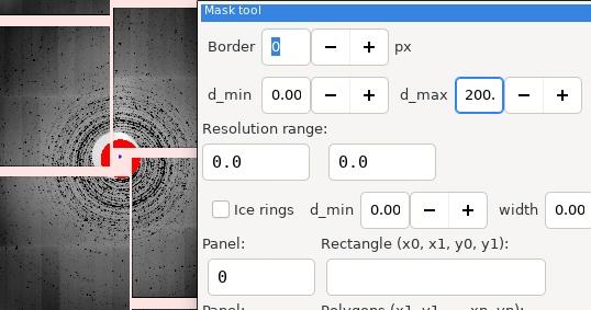
2. Beam center with a circle and mask by resolution range Open the Mask tool as shown in the previous step. From my own exploration, it doesn’t look like the Mask tool in dials.image_viewer GUI supports cross-panel geometry shape definition.
   If the actual beam center is close to the what dials have (shown by the blue cross, default to image center I believe), you can hack by using resolution range masking. For example, make d_max 200.0:

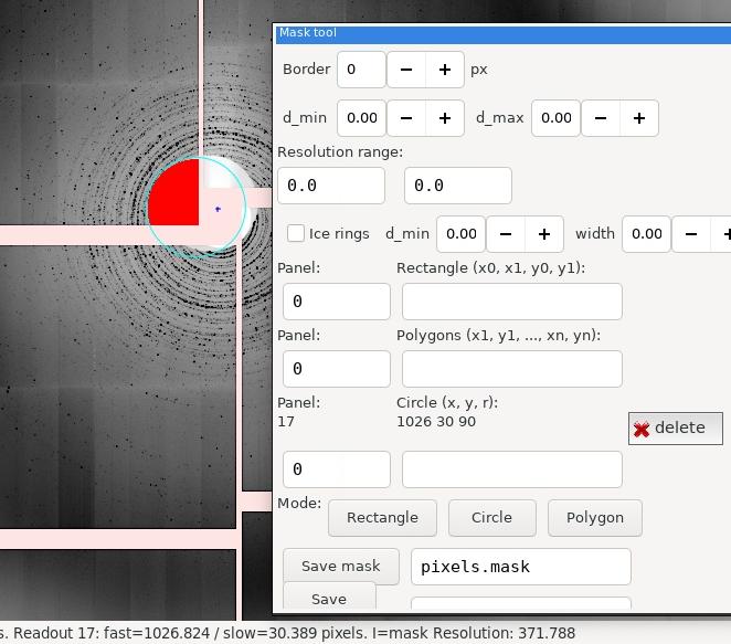
However, as you can see in this case, the beam center is actually quite shifted. If you want to define an arbitrary circle, you will see that you have to define the circle center within a particular panel, and only the circle on that panel is masked:

In this case, I typed panel 17 and defined the circle (x,y,r) as 1026,30,90. I eyeballed the radius as 90 and got the panel and the position values by hovering my mouse over the

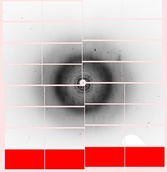
center, and at the bottom of the image you will see some text like “… Readout 17: fast=1026 / slow = 30 …”. 3. Whole panel due to shadow The easiest way to mask whole panels is actually using a command line tool. In this case, suppose I want to mask out the bottom panels which are panel 0-3 (judging from the “Readout” number as shown above). In the terminal:

dials.generate_mask out/std.cbf untrusted.panel=0 untrusted.panel=1 

untrusted.panel=2 untrusted.panel=3 output.mask=panel.mask Visually verify if this mask looks good:

If the mask is good, combine this mask with your mask from other step (such as dead pixels) using the same tool:

dials.generate_mask r0016_stddev.mask panel.mask output.mask=combined.mask 

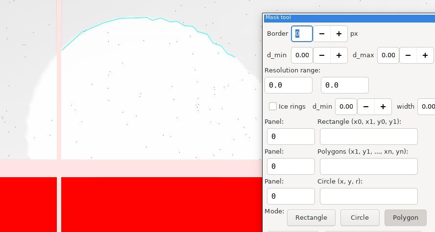
4. Irregular shape The easiest way to make a polygon mask is by clicking where the vertices would be on an image. First open the Mask tool as shown step 1.

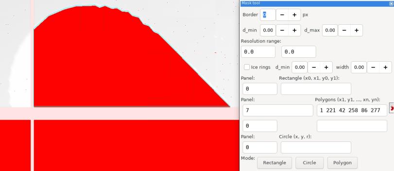
Click the Polygon button, and then if you click anywhere on the image, wherever you click would be the vertices. The order matters. Your trace / the edges of the polygon is shown as the cyan clines:

Once you roughly close the shape, click the Polygon button again, and that should properly close the polygon shape for you and mask the region:

5. Good practice notes After you think you have made a decent mask by combining some of the steps above, you can save the final mask by clicking “Save mask”.
   Below that button, you can also save the phil parameters of the masking you did through the image_viewer Mask tool, such as making a polygon mask. I strongly recommend you save this every time (change the file name to avoid overwriting) before you close the image_viewer (which you might need to open and close multiple times during a real processing). This is a quantitative way of recording you manual masking and helps reproduce.

Figures (from PDF)

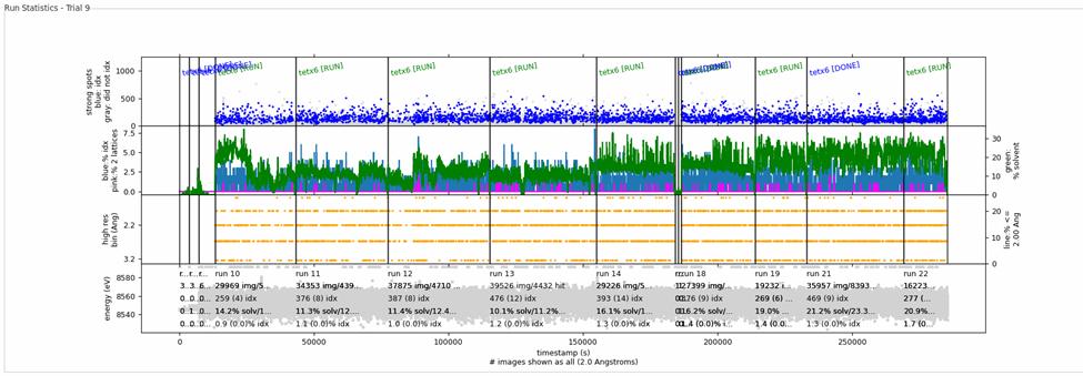
Diagnostics “Run Stats” tab of the GUI

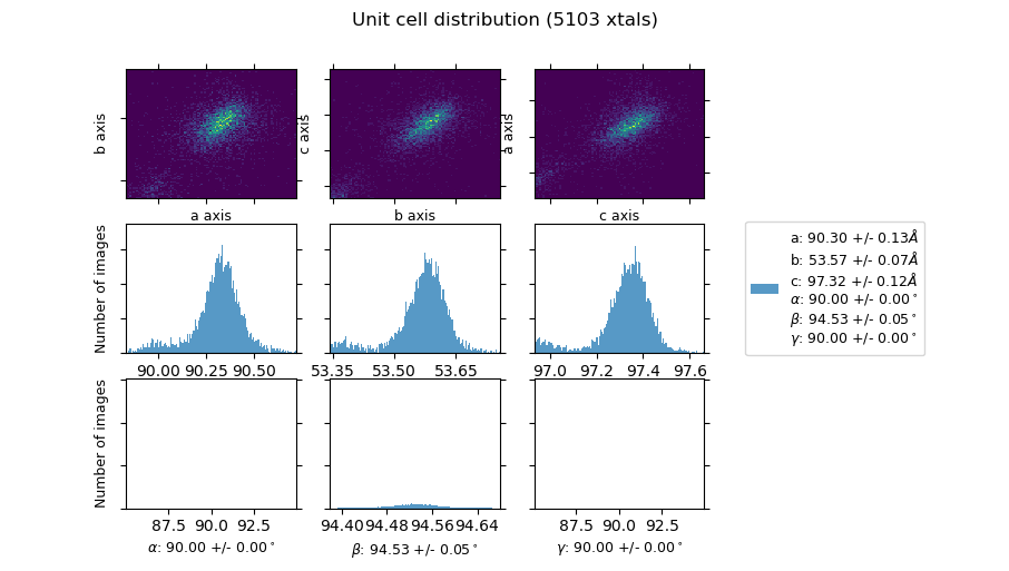
You might need to hide Options to see the numbers at the bottom. “%xtal” (behind the %solv) is the hit rate and “%idx” is the indexing rate (also plotted as the blue line in the middle panel). The numbers in the parenthesis are number of images with multiple lattices. I would also look at the top panel, where blue dot is indexed and grey dot is not, and ideally there are quite a bit of blue on top without too much grey stuff visible. It is possible to click on the dots to launch the corresponding image via dials.image_viewer to see if indexing and spotfinding works as expected. “Unit Cell” tab of the GUI

Ideally we should see nice and narrow Gaussians centered at expected cell parameters. Low indexing rate Is your spot finding good? Are there clearly visible spots that are strong and lattice-like but not picked up somehow? - Do you need to make a better mask? - Explore via dials.image_viewer on the parameters for thresholding pixels Once confirmed strong spots are found, explore indexing related knobs: - Indexing algorithm parameters: consider using indexing.stills.method_list=fft1d fft3d real_space_grid_search to your phil parameter (trial definition or run group extra phil parameter).
- Geometry: o Perform geometry refinement at both level 0 and 1. Could also explore different choices (mcd, tukey, sauter_poon) for reflections.outlier.algorithm o Try proceed to the Ensemble refinement task for updated cell and geometry Strange unit cell distribution If the unit cell distribution shape is not a nice Gaussian (but skewed or bimodal): - Do you need to (further) refine the geometry? - Was there energy drift?

• Is there indexing ambiguity for this space group + unit cell?

Figures (from PDF)

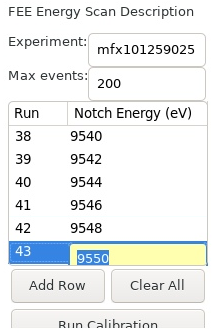
Correct energy can help indexing. To perform energy calibration, go to the “Energy” page of the GUI. 0. Populate the table On the upper left panel, click “Add Row”, then click on each entry under “Run” and “Notch Energy” to manually fill a value. (You need to click “Add Row” for each new row to add.)

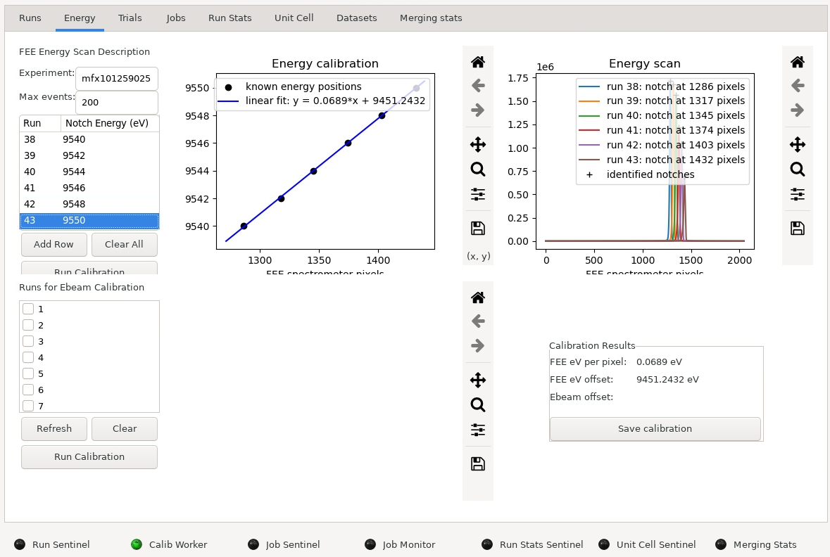
Only support one energy per run rather than a scan where many energies within a run. 1. Run Calibration Once done, click “Run Calibration.” At the bottom, the sentinel for “Calib Worker” should turn yellow indicating work in progress. This would take a few seconds, and once done, the sentinel becomes green, and you should see something like this:

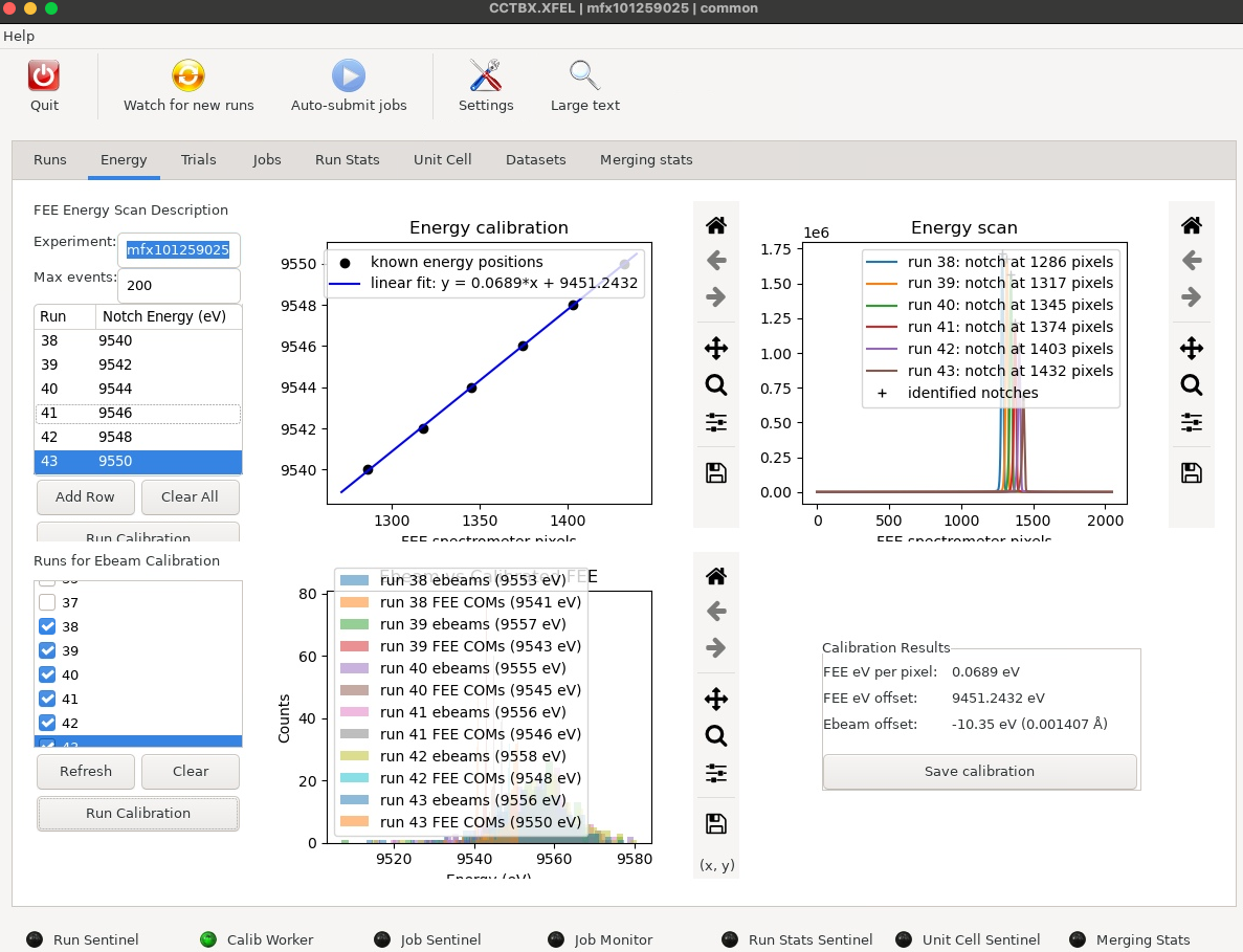
Select the same runs for Ebeam Calibration (lower left panel) and click “Run Calibration.” This can take a few minutes. Once it’s done, you should see another plot “Ebeam vs Calibrated FEE” populated and the value for “Ebeam offset” value should also be there under “Calibration results”:

If for some reason the job failed and the sentinel is red, clicking anything on this page might not get a response. After you make you corrections, you can try switch to a different page like “Trials” and then switch back to “Energy” to properly refresh the sentinel.
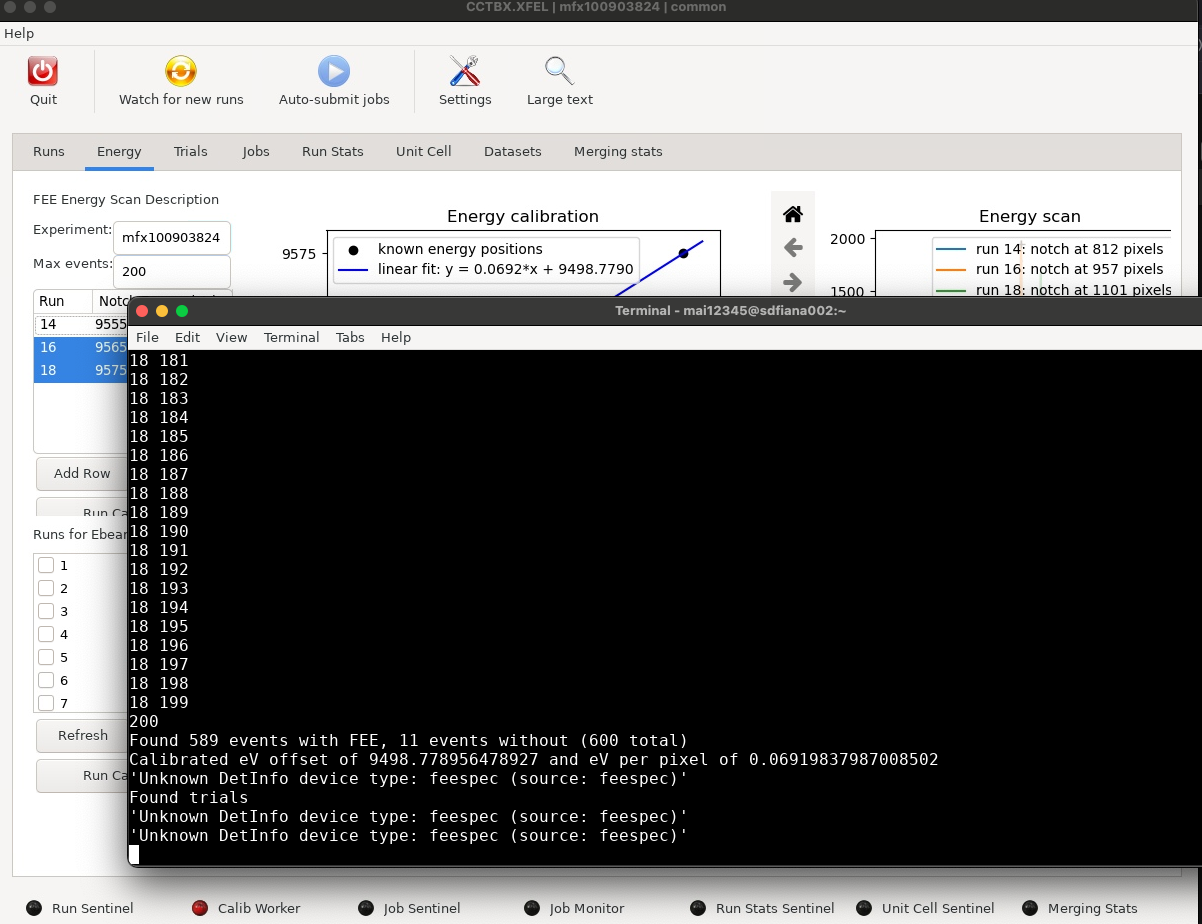
I am having trouble with other experiments for the “Ebeam Calibration.” For mfx100903824 (psana1), run 4-8 throws error on the terminal that these runs are not in any run group. For run 14, 16, and 18, I see the following error on the terminal: ‘Unknown DetInfo device type: feespec (source: feespec)’. Unclear why and how to solve it. I am having trouble with other experiments for the “Energy Calibration.” For mfx101262725 (psana2), run 225-234, I get the following error on the terminal: unsupported operand type(s) for /=: ‘NoneType’ and ‘int’. Unclear why and how to solve it. 2. Use the results for run group definition The calibration results are shown at the lower right panel, which you can save to a file if you click the button, and the file looks like this:
(base) [mai12345@sdfiana026 phils]$ cat fee_calib.phil spectrum_eV_per_pixel=0.0689

spectrum_eV_offset=9451.2432 ebeam_eV_offset=-10.35

Enter the two spectrum_eV related values when defining the run group (scroll down to see the corresponding entries in the GUI).

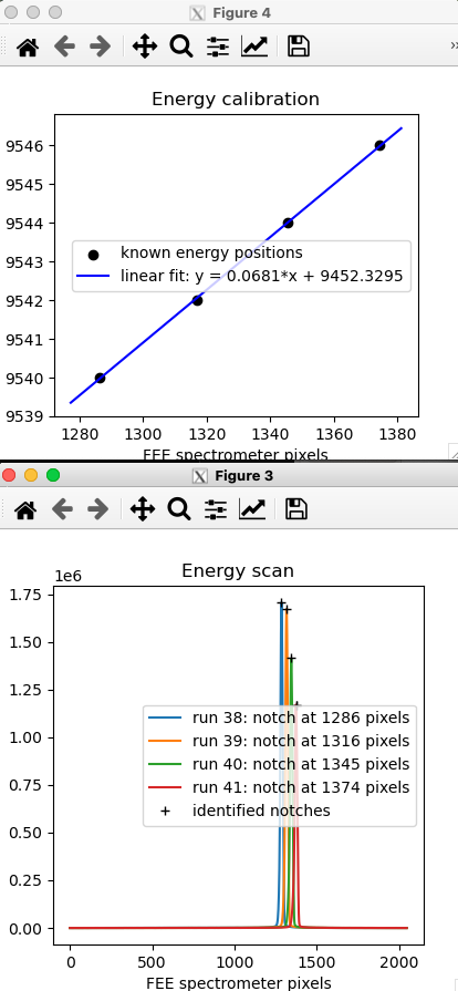
Alternative method In case something goes wrong with the GUI, the corresponding command line tool for FEE calibration is xfel.fee_calib :. For example: [mai12345@sdfiana003 ~]$ xfel.fee_calibration experiment=mfx101259025 38:9540 39:9542 40:9544 41:9546 Processing run 38… Found 1000 events with FEE, 0 events without (1000 total) Processing run 39… Found 2000 events with FEE, 0 events without (2000 total) Processing run 40… Found 3000 events with FEE, 0 events without (3000 total) Processing run 41… Found 4000 events with FEE, 0 events without (4000 total)

Calibrated eV offset of 9452.329454096232 and eV per pixel of 0.06813544632577721 wrote calibrated values to fee_calib.out [mai12345@sdfiana003 ~]$ cat fee_calib.out using experiment=mfx101259025 38:9540 39:9542 40:9544 41:9546, eV_offset=9452.329454096232 eV_per_pixel=0.06813544632577721

The command should also pop out familiar figures like this:

Figures (from PDF)

Helpful past experiments to look at include mfxl1015222 – Lane and mfx101262725 – Follmer (and other T-jump experiments in the past). If there are issues that require addressing CCTBX source code, dxtbx/src/dxtbx/format/FormatXTC.py is a key file to look at. Sanity check if event code is set up properly for a run Tthe following script list_event_codes.py by Fred is helpful: from psana import DataSource from sys import argv

args = argv[1:] exp = str(args[0]) run = int(args[1]) event_codes = [int(arg) for arg in args[2:]]

ds = DataSource(exp=exp, run=run, detectors=[‘timing’], max_events=100) myrun = next(ds.runs()) timing = myrun.Detector(‘timing’) for nevt,evt in enumerate(myrun.events()): allcodes = timing.raw.eventcodes(evt) evtcodes = [i for i, val in enumerate(allcodes) if val != 0] print(evtcodes)

To use this script, make sure you have activated psana2 environment, and then:

python list_event_codes.py <exp> <run> 

To understand the output, for example, event code 201-213 (except for 208) was set up for this T-jump experiment, and the first few line of results look like this: (ps_20241122) [mai12345@sdfiana002 dorismai]$ python list_event_codes.py mfx101262725 121 [0, 1, 9, 10, 40, 41, 42, 84, 88, 99, 101, 119, 122, 123, 128, 132, 135, 137, 140, 141, 142, 151, 152, 153, 155, 157, 158, 165, 201] [0, 1, 9, 10, 11, 40, 84, 89, 99, 101, 119, 122, 123, 128, 132, 135, 137, 140, 151, 152, 153, 155, 157, 158, 202] [0, 1, 9, 10, 40, 41, 84, 89, 99, 101, 119, 122, 123, 128, 132, 135, 137, 140, 141, 151, 152, 153, 155, 157, 158, 165, 203]

[0, 1, 9, 10, 11, 12, 13, 14, 15, 16, 40, 84, 88, 119, 122, 123, 128, 132, 135, 137, 140, 151, 152, 153, 155, 157, 158, 204] [0, 1, 9, 10, 40, 41, 42, 43, 44, 45, 46, 84, 88, 99, 101, 119, 122, 123, 128, 131, 132, 135, 137, 140, 141, 142, 143, 144, 145, 146, 149, 151, 152, 154, 155, 157, 158, 159, 165, 169, 205] [0, 1, 9, 10, 11, 40, 84, 88, 99, 101, 119, 122, 123, 128, 132, 135, 137, 140, 151, 152, 153, 155, 157, 158, 206] You can see that the last number of each shot (each array) iterates among 201 to 213 as expected. Specify event code in cctbx You can filter to process data associated with only one event code by providing “Extra XTC format parameters” when defining a run group.
For example, for the T-jump experiment mfx101262725, event code 203 is reserved for the laser ON status. To process data associated laser on, you would put in the following lines:

filter.evr_address=evr0 
filter.required_present_codes=203 

These lines are added in addition to the other lines you might need, such as “mode=psana2_idx” for psana2 data.

When tweaking PHIL parameters, it can be helpful to know what knobs are available. The command to do it is [program name] -ca 2 -e 10
Programs directly related to processing are: dials.stills_process (for Indexing task) dials.combine_experiments (for Ensemble Refinement) cctbx.xfel.merge (for Scaling and Merging tasks) There are many other programs this handbook mentioned for diagnostics or other assisting purposes, such as dials.image_viewer and cctbx.xfel.detector_residuals.

Review all the red warning texts listed previously in this document that begin with , as the resulting errors are not necessarily covered here. Failed/red sentinel / unresponsive GUI Sometimes if a particular page of the GUI goes wrong (indicated by the red sentinel), it can become unresponsive. For example, in this case the ebeam calibration has errors and “Calib Worker” sentinel becomes red:

You might get away by switching to another page (e.g. “Trials”) and then come back to “Energy” page to re-run the calibration work. No jobs submitted Error: Multiple lines on the terminal like: Warning, expected to find submitted [xxx] job: trial [xxx], rungroup[xxx], run [xxx]

Solution: Check if you have properly defined the chain of tasks under the active dataset. In particular, did you have Indexing listed first? If Indexing task was there, did it have integrate=False under the trial definition? If that’s the case, you either need another indexing task that does integration or have ensemble refinement task here. Look at parameters available to tweak for dials programs [dials progam name] -ca 2 –e 10 is a good place to start. Look at some example diffraction images You can look through the raw images using dials.image_viewer data.loc load_models=False. And remember data.loc is just specifying parameters for psana, so you can make one from scratch / modify from another data.loc file rather than waiting for the GUI indexing task to generate for you. 0. Source the right cctbx environment. If necessary, maybe also check if that it was built in the right psana environment. 1. Make a data.loc file if you don’t already have one. An example file with minimal entries look like this: experiment=mfx101262725 run=532 detector_address=jungfrau mode=psana2_idx # only for psana2 This is only a minimal set of entries. You might need other things like specifying wavelength fallback and spectrum address etc. depending on the errors you get when launching dials.image_viewer. Refer to “Check FormatXTC and data.loc” section below (and maybe also “Check psana detnames output” section). 2. Launch images via the terminal:

dials.image_viewer data.loc load_models=False 

This command lets you see the unindexed images of a run.
To look at indexed images, you would replace data.loc with the paths to the corresponding .expt and .refl files in the command. For example:

 dials.image_viewer out/idx-050_*.{expt,refl} load_models=False 

If you encounter errors with dials.image_viewer, refer to the “Dials.image_viewer related issues” section below.

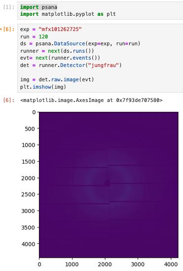
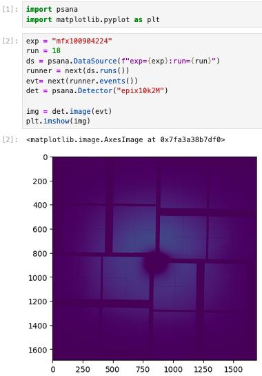
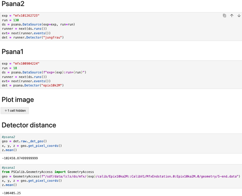
Visualize directly through psana in Jupyter Notebook Not recommended, as it is very inefficient, but if you must do this for some reason, open a jupyter notebook through ondemand interactive session, and use the following code snippets depending on psana version. Psana2 (left) Psana1 (right)

Check psana detnames output This can be useful to check if entries are missing (e.g. eBeam), and correct names of detector/spectrum addresses to access XTC files via data.loc (either manually added or provided as “Extra xtc format parameters” in the GUI) or custom psana code. For psana1: detnames exp=:run= For psana2: detnames exp=,run= Psana2 have additional flags to enable looking at scan data for example.

Check FormatXTC and data.loc Failure of this can manifest as failed to submit indexing jobs, as well as failure to open dials.image_viewer. FormatXTC is a script in cctbx:
dxtbx/src/dxtbx/format/FormatXTC.py. All the solutions below that involve manually editing data.loc file are just for debugging purposes. To properly generate the data.loc file, remember to enter the lines into cctbx.xfel GUI run group definition as “Extra xtc format parameters”. Spectrum/Detector address – 2025/11: Error: Traceback (most recent call last): File “/sdf/group/lcls/ds/tools/cctbx/psana1/build/../modules/dials/src/dials/command_line/i mage_viewer.py”, line 213, in run() File “/sdf/group/lcls/ds/tools/cctbx/psana1/conda_base_psana1/lib/python3.11/contextlib.py “, line 81, in inner return func(args, *kwds) ^^^^^^^^^^^^^^^^^^^ File “/sdf/group/lcls/ds/tools/cctbx/psana1/build/../modules/dials/src/dials/command_line/i mage_viewer.py”, line 209, in run show_image_viewer(params=params, reflections=reflections, experiments=experiments) File “/sdf/group/lcls/ds/tools/cctbx/psana1/build/../modules/dials/src/dials/command_line/i mage_viewer.py”, line 174, in show_image_viewer wrapper.display(experiments=experiments, reflections=reflections) File “/sdf/group/lcls/ds/tools/cctbx/psana1/modules/dials/src/dials/util/image_viewer/spotfin der_wrap.py”, line 86, in display self.frame.load_image(chooser_wrapper(imagesets[0], 0)) File “/sdf/group/lcls/ds/tools/cctbx/psana1/modules/dials/src/dials/util/image_viewer/spotfin der_frame.py”, line 657, in load_image super().load_image( File “/sdf/group/lcls/ds/tools/cctbx/psana1/modules/dials/src/dials/util/image_viewer/slip_vi ewer/frame.py”, line 438, in load_image self.pyslip.tiles.set_image( File “/sdf/group/lcls/ds/tools/cctbx/psana1/modules/dials/src/dials/util/image_viewer/slip_vi ewer/tile_generation.py”, line 70, in set_image self.raw_image.set_image_data(get_image_data(self.raw_image)) ^^^^^^^^^^^^^^^^^^^^^^^^^^^^^^ File “/sdf/group/lcls/ds/tools/cctbx/psana1/modules/dials/src/dials/util/image_viewer/spotfin der_frame.py”, line 851, in get_image_data image_data = image.get_image_data() ^^^^^^^^^^^^^^^^^^^^^^ File “/sdf/group/lcls/ds/tools/cctbx/psana1/modules/dials/src/dials/util/image_viewer/slip_vi

ewer/frame.py”, line 57, in get_image_data return self.image_set.get_corrected_data(self.index) ^^^^^^^^^^^^^^^^^^^^^^^^^^^^^^^^^^^^^^^^^^^^^ File “/sdf/group/lcls/ds/tools/cctbx/psana1/modules/dxtbx/src/dxtbx/imageset.py”, line 290, in get_corrected_data return super().get_corrected_data(index) ^^^^^^^^^^^^^^^^^^^^^^^^^^^^^^^^^ File “/sdf/group/lcls/ds/tools/cctbx/psana1/modules/dxtbx/src/dxtbx/format/FormatMultiIma ge.py”, line 47, in read return format_instance.get_raw_data(index) ^^^^^^^^^^^^^^^^^^^^^^^^^^^^^^^^^^^ File “/sdf/group/lcls/ds/tools/cctbx/psana1/modules/dxtbx/src/dxtbx/format/FormatXTCEpix. py”, line 38, in get_raw_data d = FormatXTCEpix.get_detector(self, index) ^^^^^^^^^^^^^^^^^^^^^^^^^^^^^^^^^^^^^^^ File “/sdf/group/lcls/ds/tools/cctbx/psana1/modules/dxtbx/src/dxtbx/format/FormatXTCEpix. py”, line 65, in get_detector return FormatXTCEpix._detector(self, index) ^^^^^^^^^^^^^^^^^^^^^^^^^^^^^^^^^^^^ File “/sdf/group/lcls/ds/tools/cctbx/psana1/modules/dxtbx/src/dxtbx/format/FormatXTCEpix. py”, line 93, in _detector wavelength = self.get_beam(index).get_wavelength() ^^^^^^^^^^^^^^^^^^^^ File “/sdf/group/lcls/ds/tools/cctbx/psana1/modules/dxtbx/src/dxtbx/format/FormatXTC.py”, line 566, in get_beam return self._beam(index) ^^^^^^^^^^^^^^^^^ File “/sdf/group/lcls/ds/tools/cctbx/psana1/modules/dxtbx/src/dxtbx/format/FormatXTC.py”, line 593, in _beam spectrum = self.get_spectrum(index) ^^^^^^^^^^^^^^^^^^^^^^^^ File “/sdf/group/lcls/ds/tools/cctbx/psana1/modules/dxtbx/src/dxtbx/format/FormatXTC.py”, line 637, in get_spectrum spectrum = self._spectrum(index) ^^^^^^^^^^^^^^^^^^^^^ File “/sdf/group/lcls/ds/tools/cctbx/psana1/modules/dxtbx/src/dxtbx/format/FormatXTC.py”, line 657, in _spectrum self._fee = psana.Detector(self.params.spectrum_address) ^^^^^^^^^^^^^^^^^^^^^^^^^^^^^^^^^^^^^^^^^^^^ File “/sdf/group/lcls/ds/tools/cctbx/psana1/conda_base_psana1/lib/python3.11/sitepackages/psana/det_interface.py”, line 58, in Detector return _detector_factory(name, env, accept_missing=accept_missing) ^^^^^^^^^^^^^^^^^^^^^^^^^^^^^^^^^^^^^^^^^^^^^^^^^^^^^^^^^^^ File “/sdf/group/lcls/ds/tools/cctbx/psana1/conda_base_psana1/lib/python3.11/sitepackages/Detector/PyDetector.py”, line 111, in detector_factory dtype = dettype(source_string, env, args, *kwargs) ^^^^^^^^^^^^^^^^^^^^^^^^^^^^^^^^^^^^^^^^^^^^ File “/sdf/group/lcls/ds/tools/cctbx/psana1/conda_base_psana1/lib/python3.11/sitepackages/Detector/PyDetector.py”, line 228, in dettype raise KeyError(‘Unknown DetInfo device type: %s (source: %s)’

KeyError: ‘Please report this error at https://github.com/dials/dials/issues or to dials-usergroup@jiscmail.ac.uk: Unknown DetInfo device type: feespec (source: feespec)’ Solution: First check psana output validity: For example, in this psana1 experiment: (ana-4.0.66-py3) [fpoitevi@sdfiana004 009_rg027]$ detnames exp=mfx100904224:run=8

---

Full Name | DAQ Alias | User Alias

FEE-SPEC0 | | MFX-DG1-BMMON | | MFX-DG2-BMMON | | NoDetector.0:Evr.0 | evr0 | MfxEndstation.0:Epix10ka2M.0 | epix10k2M | ControlData | |

---

This means in the data.loc file, add a line: spectrum_address=FEE-SPEC0 Missing eBeam – 2025/11 Error: Traceback (most recent call last): File “/sdf/group/lcls/ds/tools/cctbx/psana1/build/../modules/dials/src/dials/command_line/i mage_viewer.py”, line 213, in run() File “/sdf/group/lcls/ds/tools/cctbx/psana1/conda_base_psana1/lib/python3.11/contextlib.py “, line 81, in inner return func(args, *kwds) ^^^^^^^^^^^^^^^^^^^ File “/sdf/group/lcls/ds/tools/cctbx/psana1/build/../modules/dials/src/dials/command_line/i mage_viewer.py”, line 209, in run show_image_viewer(params=params, reflections=reflections, experiments=experiments) File “/sdf/group/lcls/ds/tools/cctbx/psana1/build/../modules/dials/src/dials/command_line/i mage_viewer.py”, line 174, in show_image_viewer wrapper.display(experiments=experiments, reflections=reflections) File “/sdf/group/lcls/ds/tools/cctbx/psana1/modules/dials/src/dials/util/image_viewer/spotfin der_wrap.py”, line 86, in display self.frame.load_image(chooser_wrapper(imagesets[0], 0)) File “/sdf/group/lcls/ds/tools/cctbx/psana1/modules/dials/src/dials/util/image_viewer/spotfin der_frame.py”, line 657, in load_image super().load_image( File

“/sdf/group/lcls/ds/tools/cctbx/psana1/modules/dials/src/dials/util/image_viewer/slip_vi ewer/frame.py”, line 417, in load_image img = rv_image(file_name_or_data) ^^^^^^^^^^^^^^^^^^^^^^^^^^^ File “/sdf/group/lcls/ds/tools/cctbx/psana1/modules/cctbx_project/rstbx/viewer/init.py”, line 248, in init detector = self._raw.get_detector() ^^^^^^^^^^^^^^^^^^^^^^^^ File “/sdf/group/lcls/ds/tools/cctbx/psana1/modules/dials/src/dials/util/image_viewer/slip_vi ewer/frame.py”, line 43, in get_detector return self.image_set.get_detector() ^^^^^^^^^^^^^^^^^^^^^^^^^^^^^ File “/sdf/group/lcls/ds/tools/cctbx/psana1/modules/dxtbx/src/dxtbx/imageset.py”, line 242, in get_detector return self._get_item_from_parent_or_format(“detector”, index) ^^^^^^^^^^^^^^^^^^^^^^^^^^^^^^^^^^^^^^^^^^^^^^^^^^^^^^^ File “/sdf/group/lcls/ds/tools/cctbx/psana1/modules/dxtbx/src/dxtbx/imageset.py”, line 236, in _get_item_from_parent_or_format item = getter_function(self.indices()[index]) ^^^^^^^^^^^^^^^^^^^^^^^^^^^^^^^^^^^^^^ File “/sdf/group/lcls/ds/tools/cctbx/psana1/modules/dxtbx/src/dxtbx/format/FormatXTCEpix. py”, line 65, in get_detector return FormatXTCEpix._detector(self, index) ^^^^^^^^^^^^^^^^^^^^^^^^^^^^^^^^^^^^ File “/sdf/group/lcls/ds/tools/cctbx/psana1/modules/dxtbx/src/dxtbx/format/FormatXTCEpix. py”, line 93, in _detector wavelength = self.get_beam(index).get_wavelength() ^^^^^^^^^^^^^^^^^^^^ File “/sdf/group/lcls/ds/tools/cctbx/psana1/modules/dxtbx/src/dxtbx/format/FormatXTC.py”, line 566, in get_beam return self._beam(index) ^^^^^^^^^^^^^^^^^ File “/sdf/group/lcls/ds/tools/cctbx/psana1/modules/dxtbx/src/dxtbx/format/FormatXTC.py”, line 627, in _beam if self._beam_cache.get_wavelength() < 0.1: ^^^^^^^^^^^^^^^^^^^^^^^^^^^^^^^
AttributeError: Please report this error at https://github.com/dials/dials/issues or to dialsuser-group@jiscmail.ac.uk: ‘NoneType’ object has no attribute ‘get_wavelength’ Solution: In the data.loc file, add a line like: wavelength_fallback=1.443 ‘NoneType’ object has no attribute ‘mode’ – 2025/11 Error: Sorry: Unable to handle the following arguments: “idx-0008_refined.expt” failed during ExperimentList processing: Traceback (most recent call last): File “/sdf/group/lcls/ds/tools/cctbx/psana1/modules/dials/src/dials/util/options.py”, line 321,

in try_read_experiments data=ExperimentListFactory.from_json_file( ^^^^^^^^^^^^^^^^^^^^^^^^^^^^^^^^^^^^^ File “/sdf/group/lcls/ds/tools/cctbx/psana1/modules/dxtbx/src/dxtbx/model/experiment_list.p y”, line 908, in from_json_file return ExperimentListFactory.from_json( ^^^^^^^^^^^^^^^^^^^^^^^^^^^^^^^^ File “/sdf/group/lcls/ds/tools/cctbx/psana1/modules/dxtbx/src/dxtbx/model/experiment_list.p y”, line 895, in from_json return ExperimentListFactory.from_dict( ^^^^^^^^^^^^^^^^^^^^^^^^^^^^^^^^ File “/sdf/group/lcls/ds/tools/cctbx/psana1/modules/dxtbx/src/dxtbx/model/experiment_list.p y”, line 885, in from_dict ).decode() ^^^^^^^^ File “/sdf/group/lcls/ds/tools/cctbx/psana1/modules/dxtbx/src/dxtbx/model/experiment_list.p y”, line 493, in decode imageset = self._imageset_from_imageset_data(imageset_data, models) ^^^^^^^^^^^^^^^^^^^^^^^^^^^^^^^^^^^^^^^^^^^^^^^^^^^^^^^^ File “/sdf/group/lcls/ds/tools/cctbx/psana1/modules/dxtbx/src/dxtbx/model/experiment_list.p y”, line 347, in _imageset_from_imageset_data imageset = self._make_stills(imageset_data, format_kwargs=format_kwargs) ^^^^^^^^^^^^^^^^^^^^^^^^^^^^^^^^^^^^^^^^^^^^^^^^^^^^^^^^^^^^^ File “/sdf/group/lcls/ds/tools/cctbx/psana1/modules/dxtbx/src/dxtbx/model/experiment_list.p y”, line 536, in _make_stills return ImageSetFactory.make_imageset( ^^^^^^^^^^^^^^^^^^^^^^^^^^^^^^ File “/sdf/group/lcls/ds/tools/cctbx/psana1/modules/dxtbx/src/dxtbx/imageset.py”, line 562, in make_imageset return format_class.get_imageset( ^^^^^^^^^^^^^^^^^^^^^^^^^^ File “/sdf/group/lcls/ds/tools/cctbx/psana1/modules/dxtbx/src/dxtbx/format/FormatMultiIma ge.py”, line 161, in get_imageset format_instance = cls.get_instance(filenames[0], format_kwargs) ^^^^^^^^^^^^^^^^^^^^^^^^^^^^^^^^^^^^^^^^^^^^^^^ File “/sdf/group/lcls/ds/tools/cctbx/psana1/modules/dxtbx/src/dxtbx/format/Format.py”, line 275, in get_instance Class.current_instance = Class(filename, kwargs) ^^^^^^^^^^^^^^^^^^^^^^^^^ File “/sdf/group/lcls/ds/tools/cctbx/psana1/modules/dxtbx/src/dxtbx/format/FormatXTCEpix. py”, line 24, in init super().init(image_file, locator_scope=epix_locator_scope, **kwargs) File “/sdf/group/lcls/ds/tools/cctbx/psana1/modules/dxtbx/src/dxtbx/format/FormatXTC.py”, line 180, in init assert self.params.mode in [ ^^^^^^^^^^^^^^^^
AttributeError: ‘NoneType’ object has no attribute ‘mode’

Solution: This is very non-descriptive error message, which is NOT referring to the mode=idx or mode=psana2_idx. Instead, I think this error shows up when you have a typo in the data.loc file. For example, it shows when I misspelled wavelength_fallback.

Dials.image_viewer related issues – 2025/11 If you encounter errors when trying to visualize images through dials.image_viewer, explore the debugging approaches below. - Check psana detnames output (see section above) - Check FormatXTC and data.loc (see section above) Check psana versions in cctbx build: In the terminal: libtbx.python -c “import psana; print(getattr(psana, ‘xtc_version’, None))” If psana1, should return None. In the terminal: libtbx.python -c “from dxtbx.format.FormatXTCEpix import FormatXTCEpix; FormatXTCEpix(‘data.loc’)” With psana1, should return no error.

Check psana geometry This can be an issue for psana2 for example, when BayFAI was deployed but the result was not successfully pushed to the database. To quickly check if psana understand the geometry correctly (is it default metrology or BayFAI) for GUI to access, you can use the following code snippets provided by Louis to check.

Database related – 2025/11 If you suspect issues related to the database, e.g. mysql error shows up in the terminal as you launch the GUI or attemp to submit jobs through the GUI, you can do some basic checking with mysql command in the terminal:

mysql -h 172.24.5.182 -u <experiment> <experiment> -p 

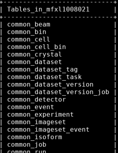
After typing password, some helpful commands to explore include (semicolon is needed): mysql> show tables;

SELECT * FROM common_job LIMIT 10; SELECT * FROM common_task LIMIT 3; Failed jobs, hanging job, and resubmit jobs – 2025/10 You might want to resubmit jobs that failed or exited but you think they should have worked (e.g. failed due to xtc file transfer not complete yet). I have also seen at reprocessing stage, a few jobs just mysteriously fail the first time submitted but second time runs fine.
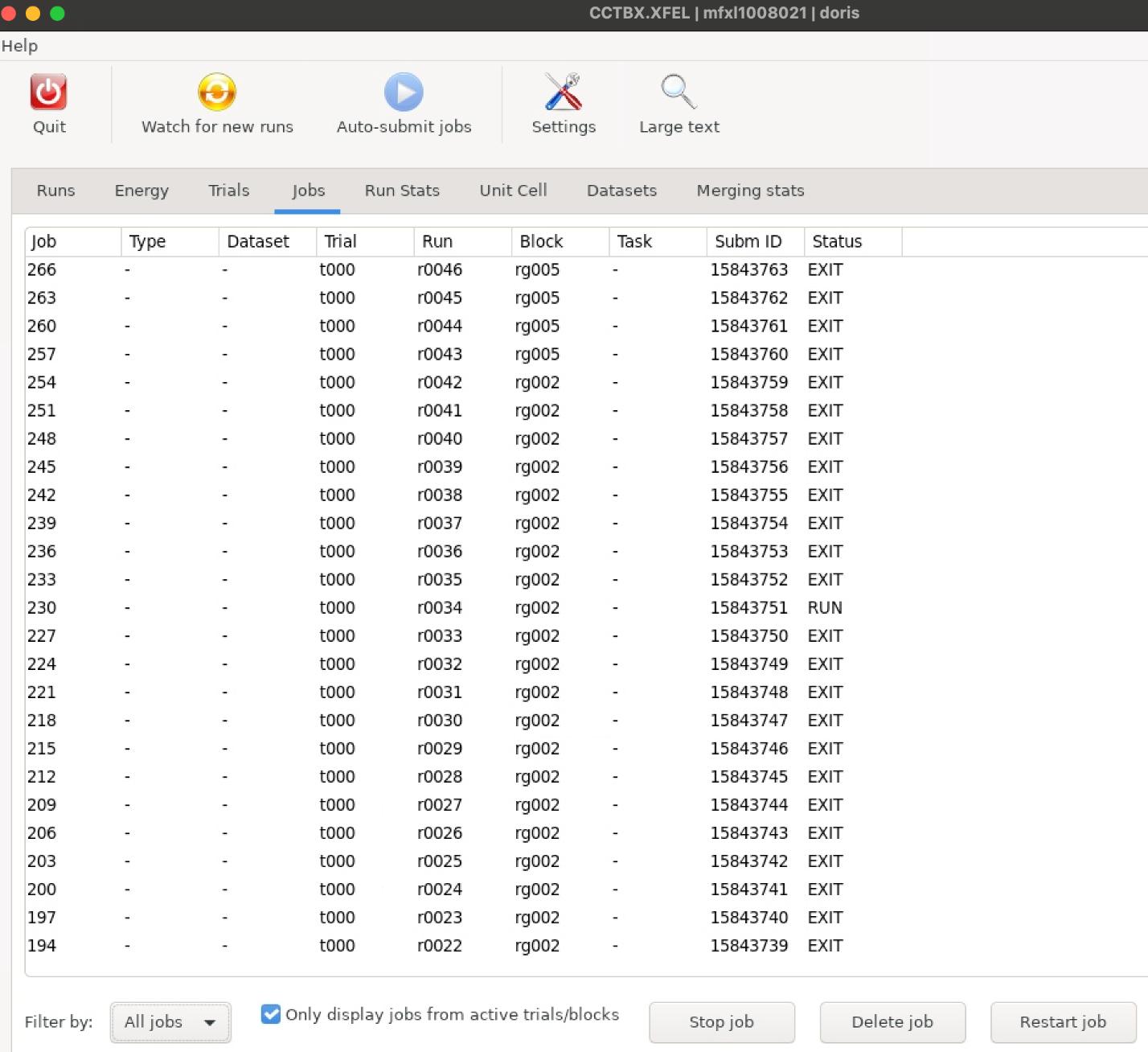
Alternatively, you might know something went wrong but the jobs haven’t finished or appear hanging forever. Typically, a cctbx job should not run more than 10 minutes. In those cases, you want to manually kill the jobs. After you see the status of a job becomes “EXIT”, you can click on that job row (or select across multiple rows) and then click “Restart job” at the bottom right. It might take a few seconds for the old job to disappear and a new job to appear (remember to have the “Autosubmit jobs” turned on).

To avoid hanging jobs due to premature start before xtc file transfer finishes, during beamtime (real-time) processing, I might sometimes disable and then re-enable “Autosubmit jobs” to create a little delay to avoid that situation. Failure to index – 2025/11 This section assumes that the indexing job cannot be submitted or cannot properly finish. If the indexing job apparently finishes without concerning errors, look at the section below “Low indexing rate” – in particular, is your initial geometry totally off?
- Are the XTC files there? This is important to check if you are reprocessing old experiments which might have data moved to tape. If there are no .xtc files directly under /sdf/data/lcls/ds/mfx/experiment_number/xtc, you need to contact

Wilko/pcds-datamgt-l email list. Once the files transfer is done, check if it has the correct permission (read for ps-data group). - Is your data.loc file correct? Is cctbx build in the right psana environment? Refer to “Check psana detnames output” and “Check FormatXTC and data.loc” sections above. A quick test is if you can successfully launch dials.image_viewer to look at some images using the GUI generated data.loc. - Are you missing ebeam and need wavelength_fallback information added to data.loc? Refer to “Check if eBeam is in xtc” section below and “Check FormatXTC and data.loc” section above.

Low indexing rate – 2025/11 - Is it a bad/short run? Do you have any image that looks like good diffraction? Identifying a few good ones is helpful for testing and improving indexing related parameters. Refer to the section “Look at some example diffraction images” above. - Do you at least have good spot finding (hit finding) rate? If not, explore those parameters first in dials.image_viewer. Refer to the chapter “Spot finding parameters exploration.” - Do you have proper masking of pixels that shouldn’t be identified as spot? Refer to the chapter “How to make a mask”. - If you have okay hit rate but low indexing rate, have you refined the geometry? Refer to the chapter “Geometry Refinement” Check if eBeam is in xtc– 2025/11 There is a helpful script from Fred (only for psana2). The command to use it is:

 python test_ebeam.py --exp <experiment> --run <run> 

The full script is attached below: from psana import DataSource import argparse parser = argparse.ArgumentParser(description=”Get a list of ebeam photon energies from psana2. Make sure you are in psana2 environment.”) parser.add_argument(‘–exp’, required=True, type=str, help=’Experiment name.’) parser.add_argument(‘–run’, required=True, type=int, help=’Run number.’) parser.add_argument(‘–nevents’, required=False, type=int, default=1000, help=’Number of events to process. Defaults to 1000.’)

args = parser.parse_args()

exp = args.exp run = args.run nevents = args.nevents

ds = DataSource(exp=exp, run=run, detectors=[‘ebeamh’], max_events=nevents) myrun = next(ds.runs()) nevent=0 damaged=0 for nevt,evt in enumerate(myrun.events()): nevent+=1 ebeam = evt.run().Detector(‘ebeamh’) hu = ebeam.raw.ebeamPhotonEnergy(evt) if hu is None: damaged+=1 else: print(hu) print(f’{damaged}/{nevent}’)

Check if event codes are in xtc – 2025/10 Similar to the script above to check ebeam, for the core piece of code, replace with follows: ds = DataSource(exp=exp, run=run, max_events=nevents) myrun = next(ds.runs()) timing = myrun.Detector(‘timing’) for nevt,evt in enumerate(myrun.events()): allcodes = timing.raw.eventcodes(evt) # make a list of indexes where allcodes is 1 usedcodes = [i for i, code in enumerate(allcodes) if code == 1] print(usedcodes) if nevt >= nevents: break

Failure to merge If merging job appears “EXIT”, is it because of no google drive publishing parameters provided (which is harmless, the job actually finished fine), or something else? Check the err.out to confirm.

Workaround (last resort) if previous processing went very wrong If something previous tasks went really wrong that prevented you from continue (e.g. submitting new tasks for new datasets), a last resort is to make a new experiment tag and start over (all the way from tagging the runs). This happened to mfxl1008021, where at some point, a custom build was used to run abismal task. In later attempts to reprocess using the official build, abismal task is not supported and considered NoneType in the processing database that prevented submitting any new task.

Figures (from PDF)

ABISMAL is a merging program for X-ray crystallography data recorded at LCLS and other XFELs. It uses deep learning and Bayesian inference and supports data processed in the CCTBX XFEL GUI used at MFX. LCLS maintains an ABISMAL installation at NERSC. Check the ABISMAL Category on the RS-Station Forum for the latest info on running ABISMAL at NERSC.